Preface
Why should I take this course?
What do you gain from taking this course? First of all, this course is based on JavaScript and Python programming languages. Language is only a technology. Finally, we should apply this technology into an industry. Quantitative trading is an emerging industry, which is currently in a rapid development stage and has a large demand for talents.
Through the systematic learning of this course, you can have a deeper understanding of the field of quantitative trading. If you are a student preparing to enter the field of quantitative trading, it will also help you. If you are a stock or futures investment enthusiast, then quantitative trading can assist your subjective trading. By developing trading strategies, you can gain profits in the financial market, and also broaden the channels and platforms for your investment and financial management.
Before that, let me talk about my personal trading experience. I am not a finance major, I studied statistics. At first, I began to trade stocks subjectively in my school days. Later, I became a quantitative trading practitioner of domestic private equity funds, mainly engaged in strategy research and strategy development.
I have been trading in this circle for more than ten years, and have developed various types of strategies. My investment philosophy is: risk control is above all else and focuses on absolute returns. The topic of our topic is: from quantitative trading to asset management – CTA strategy development for absolute return.
1. Futures CTA strategy money-making logic
1.1 Understanding Futures CTA
Someone may ask what CTA is? What exactly is the CTA? CTA is called commodity trading advisors in foreign countries and investment manager in China. The traditional CTA is to collect the funds of the majority of investors, then entrust them to professional investment institutions, and finally invest in stock index futures, commodity futures, and treasury bond futures through trading advisers (namely CTA).
But in fact, with the continuous development and expansion of the global futures market, the concept of CTA is also expanding, and its scope is far beyond traditional futures. It can invest not only in the futures market, but also in the interest rate market, the stock market, the foreign exchange market and the option market. As long as there is a certain amount of historical data for this variety, it can develop corresponding CTA strategies based on these historical data.
As early as the 1980s, the electronic trading technology was not mature. At that time, most traders judged the future trend of commodity futures by drawing technical indicators manually, such as William index, KDJ, RSI, MACD, CCI, etc. Later, traders set up a special CTA fund to help customers manage assets. It was not until the popularization of electronic trading in the 1980s that the real CTA fund began to appear.
Changes in CTA fund management size
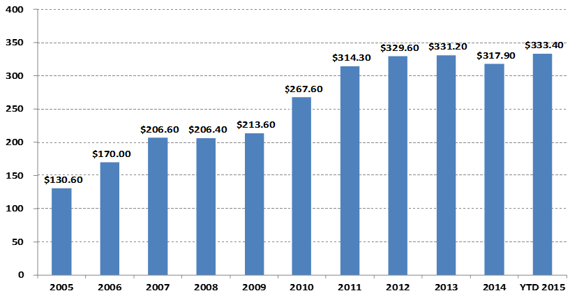
In billions of dollars
Let’s look at the chart above. Especially with the rise of quantitative trading, the scale of global CTA funds has increased from US $130.6 billion in 2005 to more than US $300 billion in 2015. CTA strategy has also become one of the mainstream investment strategies of global hedge funds.
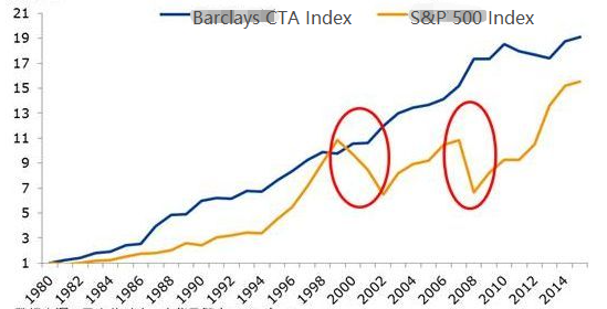
Rising alongside the size is the performance of CTA funds. Let’s look at the Barclays CTA index in the chart below. The Barclay CTA index is a representative industry benchmark for global commodity trading advisers. From the end of 1979 to the end of 2016, the cumulative return of the Barclay CTA Fund Index was up to 28.95 times, the annualized return was 9.59%, the Sharp ratio was 0.37, and the maximum withdrawal was 15.66%.
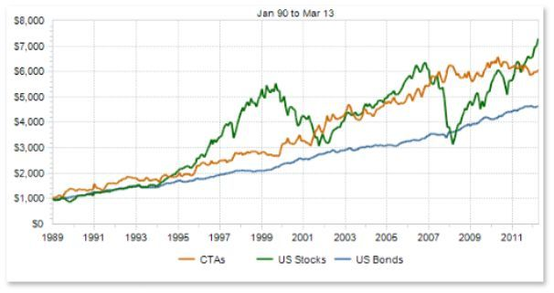
Because in the asset allocation portfolio, the CTA strategy usually maintains very low correlation with other strategies. As shown in the red circle below, during the global stock bear market from 2000 to 2002 and the global subprime crisis in 2008, the Barclay CTA fund index not only did not fall but also achieved positive returns. When the stock market and bond market were in crisis, CTA could provide strong returns. In addition, we can see that the profit level of the Barclay Commodity CTA Index since 1980 has been stronger than the S&P 500, and the withdrawal is also much lower than the S&P 500.
The development of CTA in China has only been in the past ten years, but the momentum is very strong. This is mostly due to the relatively open trading environment of domestic commodity futures, the low threshold of trading funds, the use of margin system to trade in both long and short positions, the low transaction costs, the more advanced technical structure of the exchange compared with stocks, and the easier system trading.
Since 2010, CTA funds have mainly existed in the form of private funds. With the gradual opening of the investment scope of the fund special account in domestic policies, CTA funds began to exist in the form of fund special account. Its more transparent and open operation mode has also become a necessary tool for more investors to allocate assets.
CTA strategies are also more suitable for individual traders than other trading strategies in terms of ease of entry, capital threshold, execution of trading strategies, and API connectivity. Domestic futures contracts are very small. For example, corn or soybean meal can be traded for thousands of yuan, and there is almost no capital threshold. In addition, because some CTA strategies come from traditional technical analysis, it is relatively easy compared with other strategies.
The design process of CTA strategy is also relatively simple. First, the historical data is processed initially, and then input into the quantitative model. The quantitative model includes the trading strategy formed by mathematical modeling, programming design and other tools, and the trading signal is generated by calculating and analyzing these data. Of course, in actual development, it is not as simple as the above chart. Here we just give you an overall concept.
1.2 Type of futures CTA strategy
From the perspective of trading strategy, CTA strategy is also diversified: it can be a trend strategy or an arbitrage strategy; It can be a large-period medium and long-term strategy, or an intraday short term strategy; The strategy logic can be based on technical analysis or fundamental analysis; It can be a subjective transaction or system transaction.
CTA strategy has different classification methods. According to the transaction method, it can be divided into subjective transaction and system transaction. The development of foreign CTA strategy is relatively advanced, and the CTA strategy of system transaction has been close to 100%. According to the analysis method, it can be divided into basic analysis and technical analysis. According to the source of income, it can be divided into trend trading and oscillatory trading.
In general, the CTA strategy accounts for about 70% of the total trading market, the trend strategy accounts for about 25%, and the counter trend or trend reversal strategy accounts for about 5%. Among them, the trend strategy with the largest proportion can be divided into high-frequency trading, intra-day trading, short- and medium-term trading, and medium- and long-term trading according to the position period.
High-frequency market making strategy
At present, there are two mainstream high-frequency trading strategies on the market: one is high-frequency market making strategy, the other is high-frequency arbitrage strategy. Market making strategy is to provide liquidity in the trading market. That is to say, in the trading market with a market maker, if someone wants to trade, the market maker must ensure that his order can be traded. If there is insufficient liquidity in the market and the order cannot be traded, the market maker must buy or sell the counterparty’s order.
High-frequency arbitrage strategy
High frequency arbitrage refers to trading two highly correlated stocks or ETF and ETF portfolio. According to the calculation method of ETF, the expected price of an ETF can be calculated in the same way. The ETF index price may subtract the ETF expected price to get a price difference. Usually, the price difference will run in a price channel. If the price difference breaks through the upper and lower channels, you can trade the price difference, wait for the return of the price difference, and earn income from it.
Intraday strategy
In the literal sense, as long as there is no position overnight, it can be called intra-day trading strategy. Due to the short holding period of intraday trading, it is usually impossible to make profits immediately after entering the market, and then leave the market quickly. Therefore, this trading mode bears low market risk. However, because the market changes rapidly in a short period of time, the intra-day strategy usually has higher requirements for traders.
Medium and long-term strategy
In theory, the longer the holding period is, the greater the strategic capacity and the lower the risk-return ratio will be. Especially in institutional transactions, because of the limited capacity of short-term strategies, large funds cannot enter and exit the market in a short period of time, more long-term strategies will be allocated. Generally, the position period is several days and months, or even longer.
CTA strategy data
Generally speaking, the CTA strategy is studied with minute, hour and daily data, which include: opening price, highest price, lowest price, closing price, trading volume, etc; Only a few CTA strategies will use Tick data, such as buy price, sell price, buy volume, sell volume and other in-depth data in L2 data.
As for the basic idea of CTA strategy, the first thing we think of is based on traditional technical indicators, because there are many public reference materials in this area, and the logic is usually simple, most of which are based on statistical principles. For example, we are familiar with various technical indicators: MA, SMA, EMA, MACD, KDJ, RSI, BOLL, W&R, DMI, ATR, SAR, BIAS, OBV, etc.
There are also some classic trading models on the market, which can also be used for reference and improved, including: multiple moving average combination, DualThrust, R-Breaker, Turtle trading method, grid trading method, etc.
All of these are trading strategies based on traditional technical analysis. The process is to extract factors or trading conditions with probability advantages according to historical data and correct trading concepts, and assume that the market will still have such laws in the future. Finally, the trading strategy is realized by code and fully automatic trading. Open positions, stop profits, stop losses, increase positions, reduce positions, etc., which generally do not require manual intervention. In fact, it is a strategy of buying the winners by using the positive autocorrelation coefficient of the price time series.
The biggest advantage of CTA strategy is that no matter whether the current market is rising or falling, it can obtain absolute returns, especially when the market is rapidly changing, or the market trend is obviously smooth, the advantage of the strategy is obvious, in short, if there is a trend, there is a gain. However, if the market is in a volatile situation or the trend is not obvious, the strategy may buy at a high point and sell at a low point, and stop the loss back and forth.
1.3 Profit principle of futures CTA strategy
The futures CTA strategy is profitable mainly because of the following points:
- 1. There is reflexivity in the price trend, which always continues in the way of trend. When investors observe that the price rises, they will follow the trend and buy, resulting in a further rise in the price. The same is true of price decreasing. Because investors are more irrational, sometimes we can see that the price rises abnormally and falls abnormally.
- 2. Each investor has an asymmetrical tolerance for the ratio of profit to loss and a different tolerance for risk. For most retail investors, they are more inclined to choose a more conservative homeopathic trading method, and the market is also more prone to the trend.
- 3. The formation of the price is determined by the transaction. It is true that the transaction is driven by people, but human nature is difficult to change. This is the reason why the fixed pattern will recur. The strategy is effective in the historical data backtesting, which indicates that it may also be effective in the future.
In addition, the trading feature of trend tracking is to lose a small amount of money when there is no market, and make great fortune when the market comes. However, people who have done trading know that the market is volatile most of the time, and only in a small amount of time is the trend market. Therefore, the trend tracking strategy has a low winning rate in trading, but the overall profit and loss of each transaction is relatively large.
Because the trend tracking strategy is unstable in terms of income, many investment institutions will use multiple varieties and strategies to build a portfolio, which will also be configured with a certain amount of reversal strategies. The reverse strategy is an autocorrelation with a negative coefficient in the time series of prices, i.e., high selling and low taking.
Correlation between CTA and traditional assets
Let’s look at the above chart. Theoretically, various strategies with different styles or relatively low correlation will sometimes the same and sometimes different trading signals at the same time when facing various changes in market prices. As multiple return curves overlap each other, the overall return is complementary, and the return curve will become more flat, thus reducing the volatility of returns.
From the above point of view, it can be concluded that it is better to develop multiple moderate sub-strategies than to develop a master strategy. How to control these strategies? Here we can learn from the random forest algorithm in machine learning. The random forest is not an independent algorithm, it is a decision framework containing multiple decision trees. It is equivalent to the parent strategy above the sub-strategy of the decision tree. The substrategy cluster is organized and controlled through the parent strategy.
Next, we need to design a parent strategy. We can evaluate the liquidity, profitability and stability of each variety in the entire commodity futures market to screen out the commodity futures variety portfolio with low volatility of earnings, and then conduct industry neutral screening, further reduce the overall volatility through the industry dispersion of the portfolio, and finally build the actual commodity futures multi-variety portfolio through market value matching for trading.
Each variety can also be configured with multi-parameter strategies, and it can select the parameter combination with good performance in the backtest. When the market trend is obvious, the multi-parameter strategies will generally perform consistently, which is equivalent to adding positions; When the market is in a volatile situation, the performance of multiple sets of parameter strategies will usually be inconsistent, so that they can hedge risks by going long or short, respectively, which is equivalent to reducing positions. This can further reduce the maximum backtest rate of the portfolio, while maintaining the overall rate of return unchanged.
2. Classic futures CTA strategy example
Newton once said: If I see further than others, it is because I stand on the shoulders of giants.
The CTA strategies publicly available on the market include the SMA strategy, the Bollinger band strategy, the turtle trading rules, the momentum strategy, the arbitrage strategy, and so on. Quantitative trading strategies have one characteristic, that is, they will slowly fail once they are made public. But this does not affect us to learn from these strategies and learn from the essence of them, so that we can solve problems on the shoulders of giants.
2.1 Analysis of futures fundamentals (inventory, basis difference, price)
The fundamental analysis does not need to care about the short-term price trend. It is believed that the value will be reflected in the price ultimately. It is more about analyzing the factors behind the price to determine how much the variety is worth. Generally, the top-down analysis method is adopted: from macro factors, variety factors and other factors.
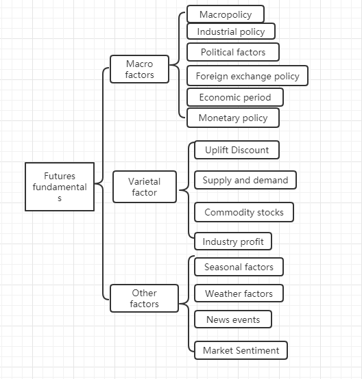
We can see from the above chart that there are many factors that affect commodity prices, and these data are changing constantly. It is beyond the ability of individual retail investors to obtain these huge data, let alone objective analysis.
In fact, the fundamental analysis of commodity futures is not to analyze all the factors. We only need to grasp the core elements of fundamental analysis to find out the rules from the complex information.
Macro factors
Macroeconomic data is complex and changeable. Every day, every moment, there are many economic data published, from national politics, central banks, investment banks, official and unofficial. In addition to the political and economic crisis, macro-analysis is a good material for chatting, but not practical. Peter Lynch, a famous fund management expert in the United States, once said: “I spend no more than 15 minutes on the analysis of the economic situation every year”.
Variety factor
In the fundamental analysis, the variety analysis is mainly to analyze premium and discount, supply and demand relationship, commodity inventory, industrial profit, etc. It can be said that mastering the variety factor analysis of commodity futures can judge most of the market trend.
As friends who have done futures know, domestic commodity futures can be simply divided into industrial products and agricultural products. The analysis methods of industrial products and agricultural products are different. We will elaborate on the two aspects of supply and demand. In industrial products, supply is relatively stable. Unless there is a major technological breakthrough, production capacity is unlikely to change significantly in a short period of time. Therefore, the main factor affecting the price of industrial products is demand. The demand for agricultural products is relatively stable. In the long run, the demand for agricultural products changes, but in the short run, the demand for agricultural products tends to be stable, so the main factor affecting the price of agricultural products is supply.
Therefore, according to the laws of economics, it is the relationship between supply and demand that determines the price of goods ultimately. In theory, as long as the data of supply and demand can be obtained, the future price of goods can be determined. For industrial products, the supply data is easy to obtain, but it is difficult to obtain the demand data. For agricultural products, the demand data is easy to obtain, and it is difficult to obtain the supply data.
In fact, we can further subtract. The mutual result of supply and demand in the economic market is inventory. We can judge the strength of the relationship between market supply and demand through inventory data. If the inventory of a commodity is very high, it means that the market supply is greater than the demand, and the commodity price will decrease on the premise that the external conditions remain unchanged. If the inventory of a commodity is very low, it means that the market demand is greater than supply, and the commodity price will increase on the premise that the external conditions remain unchanged.
In addition to analyzing commodity inventory, we also need to analyze the price difference between the spot market and the futures market, which is also called the basis difference. If the futures price is greater than the spot price, we call it the futures premium; If the futures price is less than the spot price, we call it the futures discount. According to the futures delivery system, on the futures delivery date, the futures price should be equal to the spot price.
Regardless of the premium or discount, due to the constraints of the futures delivery system, the futures price on the delivery date should be equal to the spot price in theory. As the delivery date approaches, both the spot price and the futures price will tend to be consistent. One is the return of futures to spot, and the other is the return of spot to futures.
According to the above principle, we can use inventory and basis difference to determine future futures prices at the same time. If the inventory of a commodity is low, and if the futures price is much lower than the spot price, we can judge that the demand of the spot market is greater than the supply, and the probability of the spot price increasing in the future is large; Also due to the futures delivery system, as the delivery date approaches, the futures price will rise, and it will be equal to the spot price. The probability of futures price increasing is greater in the future.
Finally, we judge the probable direction of the future price through the inventory and basis difference, but there is no accurate point of buying and selling, so we need to cooperate with technical analysis to give a clear signal of entry and exit. The structure of the whole fundamental analysis is: low inventory + deep discount + technical analysis long position signal = go long; High inventory + substantial premium + technical analysis short position signal = go short.
2.2 Turtle trading rules
When it comes to trading strategies, we have to talk about the representative turtle trading rules. The turtle trading rule comes from the most famous experiment in the history of trading. Richard Dennis, a commodity speculator, wants to know whether great traders are born or trained. To this end, in 1983, he recruited 13 people and taught them the basic concepts of futures trading, as well as his own trading methods and principles. These students were called “turtles”.
In the following four years, the Turtles achieved an average annual compound interest of 80%. Dennis proved that with a simple system and rules, people with little or no trading experience can become excellent traders. However, some turtles sell turtle trading rules on the website for profit. In order to prevent this behavior, two original turtles, Curtis Firth and Arthur Maddock, decided to make the turtle trading rules available to the public free of charge on the website.
After the truth came out, people found that the Turtle trading rules adopted the optimized Donchian channel and used ATR indicators for position management. After decades of historical tests, it has become an easy trading method for ordinary retail investors to make profits. It still works today in some varieties.
Turtle core principles
- Mastering advantages: find a trading strategy with positive expectations, because in the long run, it can create positive returns.
- Manage risk: control risk and hold your position, otherwise you may not wait for a day to make profits.
- Perseverance: Only by unswervingly implementing your strategy, can you truly achieve systematic results.
- Simple and clear: In the long run, simple systems have more vitality than complex systems.
So next, let’s see what the Turtle trading rules say.
- Market – what to buy and sell, essentially in which markets to trade. Turtles are futures traders. They choose the markets with large trading volume and high liquidity only. Because choosing the markets with inactive trading will increase the extra slippage of entry and exit, and will also miss many opportunities of trend.
- Position size – how much to buy or sell is a very important part of the whole strategy, which is usually ignored or wrongly treated by most people. The Turtle trading rule adopts ATR, that is, the average real volatility index, to calculate the open position, increase position signal and stop loss signal. This is a very ingenious design. The original intention is to adjust the size of the position through the absolute volatility of the market. When the market volatility is strong, reduce the position, and when the market volatility is weak, increase the position. It first defines a unit whose formula is: (total assets * 1%)/ATR. The initial position is 1 unit. Even if the decline of the variety on that day reaches the level of ATR, the loss on that day can be controlled within 1% of the total asset. If the price rises by 0.5 unit, the long position will increase their positions by 1 unit, up to 4 units.
- Market entry – Turtle’s market entry is based on the Donchian channel. When the price rises above the highest price of the first 20 or 55 K lines, it will enter the market to go long. When the price falls below the lowest price of the first 20 or 55 K lines, it will enter the market to go short. When the signal appears, enter the market for trading, without waiting for the close or the next K-line.
- Stop loss – In the long run, transactions that do not stop loss will not succeed, but most traders are holding loss positions and trying to take chances to hope that the market will turn over. Turtle rules stipulate when to withdraw from the loss position strictly. If you hold long position orders and the price drops by 2 units, the long position is closed with a stop loss. If you hold a short position order and the price rises by 2 units, the short position will be closed with a stop loss.
- Stop profit – In Turtle rules, stop profit means losing a lot of floating profits, which is also an unacceptable part for many traders. If you currently hold long position orders and the price falls below the track of the Donchian channel of ten days, close all long orders; If the current short position order is held and the price rises above the track of the Donchian channel of ten days, close all short positions.
Thus we can see that although the Turtle trading rules look very simple, in fact it has formed a real sense of the prototype of the trading system. It covers all aspects of a complete trading system, leaving no room for traders to make subjective imaginative decisions, which just makes the advantages of programmed operation of the system play, including: entry and exit rules, fund management and risk control, etc.
The biggest advantage of the turtle trading method is to help us establish a set of effective trading methods. It is a combination of batch opening, dynamic stop profits and stop loss, and the trend following strategy of the market, especially the use of ATR value and the concept of position management, which is very worth learning. Of course, it also has a common problem with trend tracking strategy, that is, floating profit and taking back. It is likely that all the floating profits gained from buying the winners will be taken out due to the following wave of sharp falls. It is very strong in the general trend, and not as good as expected in the volatile market.
3. Develop futures CTA strategy in practice
3.1 Development of CTA trend strategy based on MyLanguage
At the end of the last century, a very amazing trading method began to prevail in the field of financial investment in the United States. After thousands of people’s practice, people found that this method has effectiveness and great practical value. At the same time, it has been recognized by many investment experts and professional traders. Until now, it can be applied to almost all financial investment fields perfectly, whether foreign exchange, gold, stocks, futures, crude oil, or index and bond, which is chaos operation method.
The word chaos refers to the description of the chaotic state of the universe originally. Its idea is that the result is inevitable, but because the existing knowledge cannot calculate the result, because the calculation itself is also changing the result, the maximum or minimum result may appear at last, but there is no inevitable result. This is very similar to the trading market. Participants also change the market when they analyze the market and buy and sell. The market has eternal variability. When the participants understand the new form of the market, the market also understands that it is recognized by the participants, so the variation occurs. And it will tend to change in the unknown direction of the participants. It has enough wisdom to prevent the participants from catching its change rules, that is, the market is not stable, and the understanding of the past of the market cannot represent the future.
The chaos operation method is a complete set of investment ideas, trading strategies and entry and exit signals, invented by Bill Williams. At present, many investors in the world adopt chaos operation to participate in market transactions. Because the development of China’s financial market lags behind, and chaos theory is also a relatively new idea, there are few people studying chaos operation methods in China. Since chaos operation method is a trading strategy with high universality and can be applied to almost all financial investment fields, including stocks, bonds, futures, foreign exchange, and digital currency, this course uses a simplified version of chaos strategy as a starting point to improve your investment interest and income.
As the name implies, the theoretical basis of chaos operation method is chaos theory, which was proposed by meteorologist Edward Lorenz. It was one of the greatest scientific discoveries at the end of the 20th century. He put forward the famous “butterfly effect”. Bill Williams applied chaos theory to the field of financial investment creatively, combined with fractal geometry, nonlinear dynamics and other disciplines, and created a series of very effective technical analysis indicators.
The entire Chaos operation method is composed of five major dimensions (technical indicators):
- Alligator
- The Fractal
- The Momentum
- Acceleration
- The Balance Line
Let’s look at the above chart. The Alligator is a set of equilibrium lines using fractal geometry and nonlinear dynamics. Its essence is to extend the exponentially weighted moving average, which is a kind of mean line, but its calculation method is slightly more complicated than the ordinary mean line. Next, let’s look at how to define the Alligator in MyLanguage:
// Parameters
N1:=11;
N2:=21;

// Defining the price median
N3:=N1+N2;
N4:=N2+N3;
HL:=(H+L)/2;

// Alligator
Y^^SMA(REF(HL,N3),N4,1);
R:=SMA(REF(HL,N2),N3,1);
G:=SMA(REF(HL,N1),N2,1);
First, we define 2 external parameters N1 and N2, and then calculate the average HL of the highest price and the lowest price according to the external parameters, and then calculate the average HL with different parameters. For teeth, it is the average of the middle period of the midline, and the jaw is the average of the large period of the midline. In this strategy, we use the jaw.
In the chaos operation method, a fractal concept is defined vividly. We can make an analogy: open the palm of the hand, with the fingers facing up, the middle finger is the upper fractal, the left little finger and the ring finger, and the right index finger and thumb respectively, represent the K-line with no record high. A basic fractal is composed of these five K-lines. Then you can define fractal with the following code:
// Fractal
TOP_N:=BARSLAST(REF(H,2)=HHV(H,5))+2;
BOTTOM_N:=BARSLAST(REF(L,2)=LLV(L,5))+2;

TOP:=REF(H,TOP_N);
BOTTOM:=REF(L,BOTTOM_N);

MAX_YRG^^MAX(MAX(Y,R),G);
MIN_YRG^^MIN(MIN(Y,R),G);

TOP_FRACTAL^^VALUEWHEN(H>=MAX_YRG,TOP);
BOTTOM_FRACTAL^^VALUEWHEN(L<=MIN_YRG,BOTTOM);
After calculating the alligator and fractal, we can write a simple chaos operation strategy based on these two conditions, and use a group of exponentially weighted moving average lines as the benchmark price for calculating the alligator and fractal index. Of course, the original chaotic operation strategy will be more complex. The code is as follows:
// If there are no current long position orders and the closing price rises above the upper fractal and the upper fractal is above the alligator, open a long position.
BKVOL=0 AND C>=TOP_FRACTAL AND TOP_FRACTAL>MAX_YRG,BPK(1);
// If there are no current short position orders and the closing price falls below the lower fractal and the lower fractal is below the alligator, open a short position.
SKVOL=0 AND C<=BOTTOM_FRACTAL AND BOTTOM_FRACTAL<MIN_YRG,SPK(1);

// Long positions are closed if the closing price falls below the jaws of the alligator.
C<Y,SP(BKVOL);
// Short positions are closed if the closing price rises above the jaws of the alligator.
C>Y,BP(SKVOL);
For ease of understanding, I wrote the detailed comments into the code directly. We can simply list the trading logic of this strategy as follows:
- Long opening position: if there are no long position orders at present, and the closing price rises below the upper fractal, and the upper fractal is above the alligator.
- Short opening position: if there are no short position orders at present, and the closing price falls below the lower fractal, and the lower fractal is below the alligator.
- Long closing position: if the closing price falls below the alligator chin.
- Short closing position: if the closing price rises above the alligator chin.
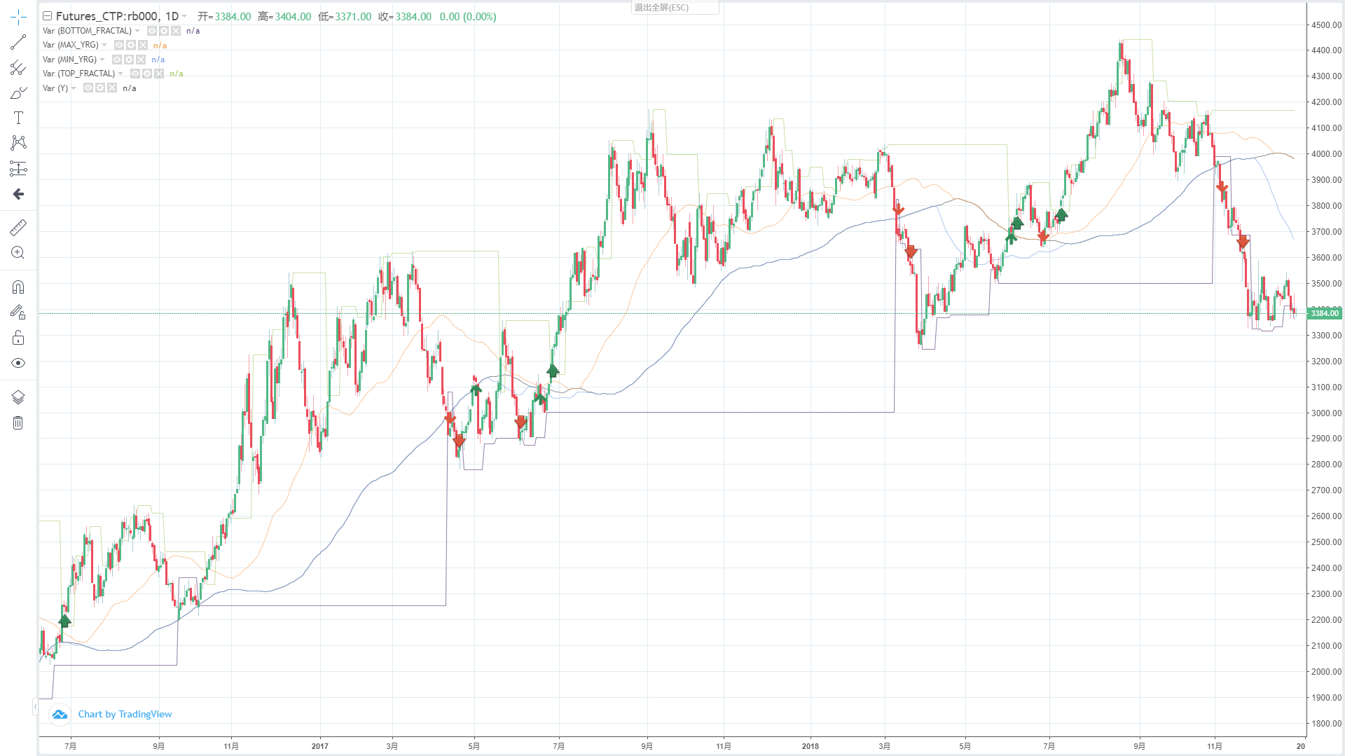
Next, let’s see what the results of this simple chaos operation strategy backtest actually look like. In order to make the backtest more close to the real market environment, the commission is set to twice the exchange rate, and the opening and closing positions are subject to a sliding point of two jumps each. The backtest data type is the rebar index, and the trading type is the rebar main force continuous, with a fixed 1 lot opening position. The following is the preliminary backtest performance report at the 1-hour level.
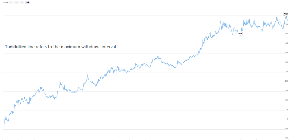
From the capital curve and backtest performance data, the strategy performed well, and the overall capital curve was steadily upward. However, since the end of 2016, the market characteristics of rebar varieties have changed, from the unilateral trend of high volatility to the broad volatility trend. From the perspective of capital curve, the profit from 2017 to now is obviously weak.
In a word, the essence of chaos operation method is to find a turning point, without caring about how the market goes or whether it is true or false breakout. If it breaks through the fractal, it will enter the market directly. Never try to predict the market, but be an observer and follower.
3.2 Development of CTA arbitrage strategy based on JavaScript language
George Soros put forward an important proposition in “The Alchemy of Finance” written in 1987: I believe the market prices are always wrong in the sense that they present a biased view of the future. He believed that the market efficiency hypothesis is only a theoretical hypothesis. In fact, market participants are not always rational, and at each time point, participants cannot completely obtain and objectively interpret all information. Moreover, even if it is the same information, everyone’s feedback is different. That is to say, the price itself already contains the wrong expectations of market participants, so in essence, the market price is always wrong. This may be the profit source of arbitrageurs.
According to the above principles, we can know that in an ineffective futures market, the reason why the market impact on delivery contracts in different periods is not always synchronous, and the pricing is not completely effective. Then, based on the delivery contract price of the same transaction object in different periods, if there is a large price difference between the two prices, we can buy and sell futures contracts in different periods at the same time for cross-period arbitrage.
Like commodity futures, digital currency also has a cross-period arbitrage contract portfolio. For example, in the OKEX exchange, there are: ETC current week, ETC next week, ETC quarter. For example, suppose that the price difference between the current week of ETC and the quarter of ETC remains around 5 for a long time. If the price difference reaches 7 one day, we expect that the price difference will return to 5 in the future. Then we can sell ETC that week and buy ETC quarter at the same time to go short the price difference, vice versa.
Although this price difference exists, there are many uncertainties in manual arbitrage due to time-consuming manual operations, poor accuracy and the impact of price changes. The charm of quantitative arbitrage lies in capturing arbitrage opportunities through quantitative models and formulating arbitrage trading strategies, as well as placing trading orders automatically to exchanges through programmed algorithms, so as to capture opportunities quickly and accurately and make profits efficiently and stably.
This course will teach you how to use the FMZ Quant Trading Platform and the ETC futures contract in the OKEX exchange to demonstrate how to capture the instantaneous arbitrage opportunities, seize the profits that can be seen every time, and hedge the risks that may be encountered in the digital currency trading with a simple arbitrage strategy.
Create a cross-period arbitrage strategy for digital currency
Difficulty: Normal
Strategy environment
- Transaction object: Ether Classic (ETC)
- Spread data: ETC current week – ETC quarter (omit cointegration test)
- Transaction period: 5 minutes
- Transaction period: 5 minutes
- Transaction type: cross period of the same type
Strategy logic
- Conditions for opening positions with going long the price difference: if the current account has no positions and the price difference is less than the lower bound of the ball, then go long the price difference. That is, buy opening positions ETC for the week, sell opening positions ETC for the quarter.
- Conditions for opening positions with going short the price difference: if there is no position in the current account, and the price difference is greater than the upper bound of the ball, then go short the price difference. That is, sell opening positions ETC for the week, buy opening positions ETC for the quarter.
- Conditions for closing positions with going long the price difference: if the current account holds going long orders of ETC in the current week and holds going short orders of ETC quarter, and the price difference is greater than the middle bound of the ball, then close long the price difference. That is, sell closing positions ETC for the week, buy closing positions ETC for the quarter.
- Conditions for closing positions with going short the price difference: if the current account holds going short orders of ETC in the current week, and holds going long orders of ETC quarter, and the price difference is less than the middle bound of the ball, then close short the price difference. That is, buy closing positions ETC for the week, sell closing positions ETC for the quarter.
The above is a simple logic description of the cross-period arbitrage strategy of digital currency. So how to implement our ideas in the program? We try to build the framework on the FMZ Quant Trading Platform.
function Data() {}  // Basic data function
Data.prototype.mp = function () {}  // Position function
Data.prototype.boll = function () {}  // Indicator function
Data.prototype.trade = function () {}  // Order placement function
Data.prototype.cancelOrders = function () {}  // Order withdrawal function
Data.prototype.isEven = function () {}  // Processing single contract function
Data.prototype.drawingChart = function () {}  // Drawing function

function onTick() {
    var data = new Data(tradeTypeA, tradeTypeB);  // Create a basic data object
    var accountStocks = data.accountData.Stocks;  // Account balance
    var boll = data.boll(dataLength, timeCycle);  // Calculate the technical indicators of boll
    data.trade();  // Calculate trading conditions to place an order
    data.cancelOrders();  // Cancel orders
    data.drawingChart(boll);  // Drawing
    data.isEven();  // Processing of holding individual contract
}

//Entry function
function main() {
    while (true) {  // Enter the polling mode
        onTick();  // Execute onTick function
        Sleep(500);  // Sleep for 0.5 seconds
    }
}
Imagine what our trading process is like in supervisory trading. There is no essential difference in system transactions. It is nothing more than acquiring data, calculating data, placing an order transaction, and processing after placing an order. The same is true in the program. First, the program will execute the main function in line 20, which is a convention. When the program completes the trading strategy preprocessing (if any), it will enter the infinite loop mode, that is, the polling mode. In the polling mode, the onTick function will be executed repeatedly.
Then in the onTick function, it is our trading process in the subjective transaction: first, obtain the basic price data, then obtain the account balance, then calculate the index, then calculate the trading conditions and place the order, and finally the processing after placing the order, including order cancellation, drawing, and processing a single contract.
The strategy framework can be easily set up according to the strategy idea and transaction process. The whole strategy can be simplified into three steps:
- Pre-processing before transaction.
- Get and calculate data.
- Place an order and deal with it later.
Next, we need to fill in the necessary detail code in the strategy framework according to the actual transaction process and transaction details.
I. Pre-processing before transaction
1. Declare the necessary global variables in the global scope.
- Declare a chart object for the configuration chart
var chart = {}
- Call Chart function and initialize the chart
var ObjChart = Chart ( chart )
- Declare an empty array to store price difference series
var bars = []
- Declare a record history data timestamp variable
var oldTime = 0
2. Configure the external parameters of the strategy.
var tradeTypeA = "this_week"; // Arbitrage A Contract
var tradeTypeB = "quarter"; // Arbitrage B Contract
var dataLength = 10; // Indicator period length
var timeCycle = 1; // K-line period
var name = "ETC"; // Currencies
var unit = 1; // Order quantity
3. Define the data processing function
- Basic data function: Data()
Create a constructor, Data, and define its internal properties. Including: account data, position data, K-line data timestamp, buy/sell price of arbitrage A/B contract, and positive/negative arbitrage price difference.
function Data(tradeTypeA, tradeTypeB) { // Pass in arbitrage A contract and arbitrage B contract
    this.accountData = _C(exchange.GetAccount); // Get account information
    this.positionData = _C(exchange.GetPosition); // Get position information
    var recordsData = _C(exchange.GetRecords); // Get K-line data
    exchange.SetContractType(tradeTypeA); // Subscription arbitrage A contract
    var depthDataA = _C(exchange.GetDepth); // Depth data of arbitrage A contract
    exchange.SetContractType(tradeTypeB); // Subscription arbitrage B contract
    var depthDataB = _C(exchange.GetDepth); // Depth data of arbitrage B contract
    this.time = recordsData[recordsData.length - 1].Time; // Time of obtaining the latest data
    this.askA = depthDataA.Asks[0].Price; // Sell one price of Arbitrage A contract
    this.bidA = depthDataA.Bids[0].Price; // Buy one price of Arbitrage A contract
    this.askB = depthDataB.Asks[0].Price; // Sell one price of Arbitrage B contract
    this.bidB = depthDataB.Bids[0].Price; // Buy one price of Arbitrage B contract
    // Positive arbitrage price differences (Sell one price of contract A - Buy one price of contract B)
    this.basb = depthDataA.Asks[0].Price - depthDataB.Bids[0].Price;
    // Negative arbitrage price differences (Buy one price of contract A - Sell one price of contract B)
    this.sabb = depthDataA.Bids[0].Price - depthDataB.Asks[0].Price;
}
- Get the position function: mp ( )
Traverse the entire position array and return the position quantity of the specified contract and direction. If not, return false.
Data.prototype.mp = function (tradeType, type) {
    var positionData = this.positionData; // Get position information
    for (var i = 0; i < positionData.length; i++) {
        if (positionData[i].ContractType == tradeType) {
            if (positionData[i].Type == type) {
                if (positionData[i].Amount > 0) {
                    return positionData[i].Amount;
                }
            }
        }
    }
    return false;
}
- K-line and indicator function: boll()
A new K-line sequence is synthesized according to the positive arbitrage/negative arbitrage price difference data. The data of upper track, middle track and lower track calculated by the boll indicator are returned.
Data.prototype.boll = function (num, timeCycle) {
    var self = {}; // Temporary objects
    // Median value of positive arbitrage price difference and negative arbitrage price difference
    self.Close = (this.basb + this.sabb) / 2;
    if (this.timeA == this.timeB) {
        self.Time = this.time;
    } // Compare two depth data timestamps
    if (this.time - oldTime > timeCycle * 60000) {
        bars.push(self);
        oldTime = this.time;
    } // Pass in the price difference data object into the K-line array according to the specified time period
    if (bars.length > num * 2) {
        bars.shift(); // Control the length of the K-line array
    } else {
        return;
    }
    var boll = TA.BOLL(bars, num, 2); // Call the boll indicator in the talib library
    return {
        up: boll[0][boll[0].length - 1], // boll indicator upper track
        middle: boll[1][boll[1].length - 1], // boll indicator middle track
        down: boll[2][boll[2].length - 1] // boll indicator down track
    } // Return a processed boll indicator data
}
- Order function: trade()
Pass in the order contract name and order type, then place the order with consideration, and return the result after placing the order. Since it is necessary to place two orders in different directions at the same time, the buy/sell one price is converted within the function according to the contract name of the order.
Data.prototype.trade = function (tradeType, type) {
    exchange.SetContractType(tradeType); // Resubscribe to a contract before placing an order
    var askPrice, bidPrice;
    if (tradeType == tradeTypeA) { // If the order is placed in contract A
        askPrice = this.askA; // set askPrice
        bidPrice = this.bidA; // set bidPrice
    } else if (tradeType == tradeTypeB) { // If the order is placed in contract B
        askPrice = this.askB; // set askPrice
        bidPrice = this.bidB; // set bidPrice
    }
    switch (type) { // Match order placement mode
        case "buy":
            exchange.SetDirection(type); // Set order placement mode
            return exchange.Buy(askPrice, unit);
        case "sell":
            exchange.SetDirection(type); // Set order placement mode
            return exchange.Sell(bidPrice, unit);
        case "closebuy":
            exchange.SetDirection(type); // Set order placement mode
            return exchange.Sell(bidPrice, unit);
        case "closesell":
            exchange.SetDirection(type); // Set order placement mode
            return exchange.Buy(askPrice, unit);
        default:
            return false;
    }
}
- Cancel Order Function: cancelOrders()
Get an array of all outstanding orders and cancel them one by one. In addition, false is returned if there is an unfilled order, and true is returned if there is no unfilled order.
Data.prototype.cancelOrders = function () {
    Sleep(500); // Delay before cancellation, because some exchanges, you know what I mean
    var orders = _C(exchange.GetOrders); // Get an array of unfilled orders
    if (orders.length > 0) { // If there are unfilled orders
        for (var i = 0; i < orders.length; i++) { // Iterate through the array of unfilled orders
            exchange.CancelOrder(orders[i].Id); // Cancel unfilled orders one by one
            Sleep(500); // Delay 0.5 seconds
        }
        return false; // Return false if an unfilled order is cancelled
    }
    return true; // Return true if there are no unfilled orders
}
- Handle holding a single contract: isEven()
In the case of a single leg in the arbitrage transaction, we will simply close all positions. Of course, it can also be changed to the tracking method.
Data.prototype.isEven = function () {
    var positionData = this.positionData; // Get position information
    var type = null; // Switch position direction
    // If the remaining 2 of the position array length is not equal to 0 or the position array length is not equal to 2
    if (positionData.length % 2 != 0 || positionData.length != 2) {
        for (var i = 0; i < positionData.length; i++) { // Iterate through the position array
            if (positionData[i].Type == 0) { // If it is a long order
                type = 10; // Set order parameters
            } else if (positionData[i].Type == 1) { // If it is a short order
                type = -10; // Set order parameters
            }
            // Close all positions
            this.trade(positionData[i].ContractType, type, positionData[i].Amount);
        }
    }
}
- Drawing function: drawingChart ( )
Call ObjChart Add () method, draw the necessary market data and indicator data in the chart: upper track, middle track, lower track, positive/negative arbitrage price difference.
Data.prototype.drawingChart = function (boll) {
    var nowTime = new Date().getTime();
    ObjChart.add([0, [nowTime, boll.up]]);
    ObjChart.add([1, [nowTime, boll.middle]]);
    ObjChart.add([2, [nowTime, boll.down]]);
    ObjChart.add([3, [nowTime, this.basb]]);
    ObjChart.add([4, [nowTime, this.sabb]]);
    ObjChart.update(chart);
}
4. In the entry function main(), execute the pre-transaction pre-processing code, which will only run once after the program is started, including:
SetErrorFilter ( )to filter the unimportant information in the consoleexchange.IO ( )to set the digital currency to be tradedObjChart.reset ( )to clear the previous chart drawn before starting the programLogProfitReset ( )to clear the status bar information before starting the program
After the above pre-transaction pre-processing is defined, the next step is to enter the polling mode and execute the onTick() function repeatedly. It also sets the sleep time for Sleep () polling, because the API of some digital currency exchanges has built-in access limit for a certain period of time.
function main() {
    // Filter the unimportant information in the console
    SetErrorFilter("429|GetRecords:|GetOrders:|GetDepth:|GetAccount|:Buy|Sell|timeout|Futures_OP");
    exchange.IO("currency", name + '_USDT'); // Set the digital currency to be traded
    ObjChart.reset(); // Clear the previous chart drawn before starting the program
    LogProfitReset(); // Clear the status bar information before starting the program
    while (true) { // Enter the polling mode
        onTick(); // Execute onTick function
        Sleep(500); // Sleep for 0.5 seconds
    }
}
II. Get and calculate data
- Obtain basic data object, account balance, and boll indicator data for use in the trading logic.
function onTick() {
    var data = new Data(tradeTypeA, tradeTypeB); // Create a basic data object
    var accountStocks = data.accountData.Stocks; // Account balance
    var boll = data.boll(dataLength, timeCycle); // Get boll indicator data
    if (!boll) return; // Return if there is no boll data
}
III. Place an order and handle the follow-up
- Execute the buying and selling operation according to the above strategic logic. First, judge whether the price and indicator conditions are valid, then judge whether the position conditions are valid, and finally execute the trade () order function.
// Explanation of the price difference
// basb = (Sell one price of contract A - Buy one price of contract B)
// sabb = (Buy one price of contract A - Sell one price of contract B)
if (data.sabb > boll.middle && data.sabb < boll.up) { // If sabb is higher than the middle track
    if (data.mp(tradeTypeA, 0)) { // Check whether contract A has long orders before placing an order
        data.trade(tradeTypeA, "closebuy"); // Contract A closes long position
    }
    if (data.mp(tradeTypeB, 1)) { // Check whether contract B has short orders before placing an order
        data.trade(tradeTypeB, "closesell"); // Contract B closes short position
    }
} else if (data.basb < boll.middle && data.basb > boll.down) { // If basb is lower than the middle track
    if (data.mp(tradeTypeA, 1)) { // Check whether contract A has short orders before placing an order
        data.trade(tradeTypeA, "closesell"); // Contract A closes short position
    }
    if (data.mp(tradeTypeB, 0)) { // Check whether contract B has long orders before placing an order
        data.trade(tradeTypeB, "closebuy"); // Contract B closes long position
    }
}
if (accountStocks * Math.max(data.askA, data.askB) > 1) { // If there is balance in the account
    if (data.basb < boll.down) { // If basb price difference is lower than the down track
        if (!data.mp(tradeTypeA, 0)) { // Check whether contract A has long orders before placing an order
            data.trade(tradeTypeA, "buy"); // Contract A opens long position
        }
        if (!data.mp(tradeTypeB, 1)) { // Check whether contract B has short orders before placing an order
            data.trade(tradeTypeB, "sell"); // Contract B opens short position
        }
    } else if (data.sabb > boll.up) { // If sabb price difference is higher than the upper track
        if (!data.mp(tradeTypeA, 1)) { // Check whether contract A has short orders before placing an order
            data.trade(tradeTypeA, "sell"); // Contract A opens short position
        }
        if (!data.mp(tradeTypeB, 0)) { // Check whether contract B has long orders before placing an order
            data.trade(tradeTypeB, "buy"); // Contract B opens long position
        }
    }
}
- After the order is placed, it is necessary to deal with the abnormal situations such as the unsettled order and the holding of a single contract. And draw the chart.
data.cancelOrders(); // cancel orders
data.drawingChart(boll); // drawing
data.isEven(); // Handle holding individual contracts
As above, we have created a simple cross-period arbitrage strategy of digital currency completely through more than 200 lines code. The complete code is as follows:
// Global variable
// Declare a chart object for the configuration chart
var chart = {
    __isStock: true,
    tooltip: {
        xDateFormat: '%Y-%m-%d %H:%M:%S, %A'
    },
    title: {
        text: 'transaction profit and loss curve (detailed)'
    },
    rangeSelector: {
        buttons: [{
            type: 'hour',
            count: 1,
            text: '1h'
        }, {
            type: 'hour',
            count: 2,
            text: '3h'
        }, {
            type: 'hour',
            count: 8,
            text: '8h'
        }, {
            type: 'all',
            text: 'All'
        }],
        selected: 0,
        inputEnabled: false
    },
    xAxis: {
        type: 'datetime'
    },
    yAxis: {
        title: {
            text: 'price difference'
        },
        opposite: false,
    },
    series: [{
        name: "upper track",
        id: "line1,up",
        data: []
    }, {
        name: "middle track",
        id: "line2,middle",
        data: []
    }, {
        name: "down track",
        id: "line3,down",
        data: []
    }, {
        name: "basb",
        id: "line4,basb",
        data: []
    }, {
        name: "sabb",
        id: "line5,sabb",
        data: []
    }]
};
var ObjChart = Chart(chart); // Drawing object
var bars = []; // Storage price difference series
var oldTime = 0; // Record historical data timestamp

// Parameters
var tradeTypeA = "this_week"; // Arbitrage A contract
var tradeTypeB = "quarter"; // Arbitrage B contract
var dataLength = 10; // Indicator period length
var timeCycle = 1; // K-line period
var name = "ETC"; // Currencies
var unit = 1; // Order quantity

// basic data
function Data(tradeTypeA, tradeTypeB) { // Pass in arbitrage A contract and arbitrage B contract
    this.accountData = _C(exchange.GetAccount); // Get account information
    this.positionData = _C(exchange.GetPosition); // Get position information
    var recordsData = _C(exchange.GetRecords); // Get K-line data
    exchange.SetContractType(tradeTypeA); // Subscribe to arbitrage A contract
    var depthDataA = _C(exchange.GetDepth); // Arbitrage A contract depth data
    exchange.SetContractType(tradeTypeB); // Subscribe to arbitrage B contract
    var depthDataB = _C(exchange.GetDepth); // Arbitrage B contract depth data
    this.time = recordsData[recordsData.length - 1].Time; // Time to get the latest data
    this.askA = depthDataA.Asks[0].Price; // Sell one price of arbitrage A contract
    this.bidA = depthDataA.Bids[0].Price; // Buy one price of arbitrage A contract
    this.askB = depthDataB.Asks[0].Price; // Sell one price of arbitrage B contract
    this.bidB = depthDataB.Bids[0].Price; // Buy one price of arbitrage B contract
    // Positive arbitrage price difference (Sell one price of contract A - Buy one price of contract B)
    this.basb = depthDataA.Asks[0].Price - depthDataB.Bids[0].Price;
    // Negative arbitrage price difference (Buy one price of contract A - Sell one price of contract B)
    this.sabb = depthDataA.Bids[0].Price - depthDataB.Asks[0].Price;
}

// Get position
Data.prototype.mp = function (tradeType, type) {
    var positionData = this.positionData; // Get position information
    for (var i = 0; i < positionData.length; i++) {
        if (positionData[i].ContractType == tradeType) {
            if (positionData[i].Type == type) {
                if (positionData[i].Amount > 0) {
                    return positionData[i].Amount;
                }
            }
        }
    }
    return false;
}

// Synthesis of new K-line data and boll indicator data
Data.prototype.boll = function (num, timeCycle) {
    var self = {}; // Temporary objects
    // Median value of between positive arbitrage price difference and negative arbitrage price difference
    self.Close = (this.basb + this.sabb) / 2;
    if (this.timeA == this.timeB) {
        self.Time = this.time;
    } // Compare two depth data timestamps
    if (this.time - oldTime > timeCycle * 60000) {
        bars.push(self);
        oldTime = this.time;
    } // Pass in the price difference data object into the K-line array according to the specified time period
    if (bars.length > num * 2) {
        bars.shift(); // Control the length of the K-line array
    } else {
        return;
    }
    var boll = TA.BOLL(bars, num, 2); // Call the boll indicator in the talib library
    return {
        up: boll[0][boll[0].length - 1], // boll indicator upper track
        middle: boll[1][boll[1].length - 1], // boll indicator middle track
        down: boll[2][boll[2].length - 1] // boll indicator down track
    } // Return a processed boll indicator data
}

// Place an order
Data.prototype.trade = function (tradeType, type) {
    exchange.SetContractType(tradeType); // Resubscribe to a contract before placing an order
    var askPrice, bidPrice;
    if (tradeType == tradeTypeA) { // If the order is placed in contract A
        askPrice = this.askA; // Set askPrice
        bidPrice = this.bidA; // Set bidPrice
    } else if (tradeType == tradeTypeB) { // If the order is placed in contract B
        askPrice = this.askB; // Set askPrice
        bidPrice = this.bidB; // Set bidPrice
    }
    switch (type) { // Match order placement mode
        case "buy":
            exchange.SetDirection(type); // Set order placement mode
            return exchange.Buy(askPrice, unit);
        case "sell":
            exchange.SetDirection(type); // Set order placement mode
            return exchange.Sell(bidPrice, unit);
        case "closebuy":
            exchange.SetDirection(type); // Set order placement mode
            return exchange.Sell(bidPrice, unit);
        case "closesell":
            exchange.SetDirection(type); // Set order placement mode
            return exchange.Buy(askPrice, unit);
        default:
            return false;
    }
}

// Cancel orders
Data.prototype.cancelOrders = function () {
    Sleep(500); // Delay before cancellation, because some exchanges, you know what I mean
    var orders = _C(exchange.GetOrders); // Get an array of unfilled orders
    if (orders.length > 0) { // If there are unfilled orders
        for (var i = 0; i < orders.length; i++) { // Iterate through the array of unfilled orders
            exchange.CancelOrder(orders[i].Id); // Cancel unfilled orders one by one
            Sleep(500); // Sleep for 0.5 seconds
        }
        return false; // Return false if an unfilled order is cancelled
    }
    return true; // Return true if there are no unfilled orders
}

// Handle holding individual contracts
Data.prototype.isEven = function () {
    var positionData = this.positionData; // Get position information
    var type = null; // Switch position direction
    // If the remaining 2 of the position array length is not equal to 0 or the position array length is not equal to 2
    if (positionData.length % 2 != 0 || positionData.length != 2) {
        for (var i = 0; i < positionData.length; i++) { // Iterate through the position array
            if (positionData[i].Type == 0) { // If it is a long order
                type = 10; // Set order parameters
            } else if (positionData[i].Type == 1) { // If it is a short order
                type = -10; // Set order parameters
            }
            // Close all positions
            this.trade(positionData[i].ContractType, type, positionData[i].Amount);
        }
    }
}

// Drawing
Data.prototype.drawingChart = function (boll) {
    var nowTime = new Date().getTime();
    ObjChart.add([0, [nowTime, boll.up]]);
    ObjChart.add([1, [nowTime, boll.middle]]);
    ObjChart.add([2, [nowTime, boll.down]]);
    ObjChart.add([3, [nowTime, this.basb]]);
    ObjChart.add([4, [nowTime, this.sabb]]);
    ObjChart.update(chart);
}

// Trading conditions
function onTick() {
    var data = new Data(tradeTypeA, tradeTypeB); // Create a basic data object
    var accountStocks = data.accountData.Stocks; // Account balance
    var boll = data.boll(dataLength, timeCycle); // Get boll indicator data
    if (!boll) return; // Return if there is no boll data
    // Explanation of price difference
    // basb = (Sell one price of contract A - Buy one price of contract B)
    // sabb = (Buy one price of contract A - Sell one price of contract B)
    if (data.sabb > boll.middle && data.sabb < boll.up) { // If sabb is higher than the middle track
        if (data.mp(tradeTypeA, 0)) { // Check whether contract A has long orders before placing an order
            data.trade(tradeTypeA, "closebuy"); // Contract A closes long position
        }
        if (data.mp(tradeTypeB, 1)) { // Check whether contract B has short orders before placing an order
            data.trade(tradeTypeB, "closesell"); // Contract B closes short position
        }
    } else if (data.basb < boll.middle && data.basb > boll.down) { // If basb is lower than the middle track
        if (data.mp(tradeTypeA, 1)) { // Check whether contract A has short orders before placing an order
            data.trade(tradeTypeA, "closesell"); // Contract A closes short position
        }
        if (data.mp(tradeTypeB, 0)) { // Check whether contract B has long orders before placing an order
            data.trade(tradeTypeB, "closebuy"); // Contract B closes long position
        }
    }
    if (accountStocks * Math.max(data.askA, data.askB) > 1) { // If there is a balance in the account
        if (data.basb < boll.down) { // If basb price difference is lower than the down track
            if (!data.mp(tradeTypeA, 0)) { // Check whether contract A has long orders before placing an order
                data.trade(tradeTypeA, "buy"); // Contract A opens long position
            }
            if (!data.mp(tradeTypeB, 1)) { // Check whether contract B has short orders before placing an order
                data.trade(tradeTypeB, "sell"); // Contract B opens short position
            }
        } else if (data.sabb > boll.up) { // If sabb price difference is higher than the upper track
            if (!data.mp(tradeTypeA, 1)) { // Check whether contract A has short orders before placing an order
                data.trade(tradeTypeA, "sell"); // Contract A opens short position
            }
            if (!data.mp(tradeTypeB, 0)) { // Check whether contract B has long orders before placing an order
                data.trade(tradeTypeB, "buy"); // Contract B opens long position
            }
        }
    }
    data.cancelOrders(); // Cancel orders
    data.drawingChart(boll); // Drawing
    data.isEven(); // Handle holding individual contracts
}

// Entry function
function main() {
    // Filter unimportant information in the console
    SetErrorFilter("429|GetRecords:|GetOrders:|GetDepth:|GetAccount|:Buy|Sell|timeout|Futures_OP");
    exchange.IO("currency", name + '_USDT'); //Set the digital currency to be traded
    ObjChart.reset(); // Clear the previous chart drawn before starting the program
    LogProfitReset(); // Clear the status bar information before starting the program
    while (true) { // Enter polling mode
        onTick(); // Execute the onTick function
        Sleep(500); // Sleep for 0.5 seconds
    }
}
Arbitrage trading originated from the stock trading strategy of Morgan Stanley. Its idea is that the price difference of two highly correlated varieties conforms to the “popcorn process”, that is, the price difference keeps returning to the mean from a position that deviates from the historical mean, and then deviates again from the mean.
Therefore, we can buy low and sell high on the price difference to gain profits. Then, according to the principle of standard deviation in statistics, the Bollinger band is formed by a middle track and the upper and lower tracks calculated by the standard deviation, the formation of three mesh band, which are very practical in the price difference arbitrage transaction.
After testing, operating according to this strategy, the overall income is relatively stable, although the income is not very much each time without considering the handling fee and impact cost. It should be noted that due to the statistical arbitrage, there is a risk of reverse expansion of the price difference. We must consider the stop-loss problem when designing. Secondly, we also need to pay attention to the impact cost. When the liquidity of the two contracts involved in the transaction shrinks, it will have a great impact on the income, and investors should avoid it as appropriate.
4. Advanced iteration of CTA strategy development
4.1 Avoid the pitfalls of futures CTA strategy
In the last two classes, we wrote a trend strategy in MyLanguage and an arbitrage strategy in JavaScript. We didn’t see any problems in the strategy backtest. However, quantitative trading is not a program, whose backtest can be done directly without any problems.
In fact, the backtest is only a simulation of the strategy. It is only used to evaluate the performance of the strategy in the historical data. It allows traders to evaluate and discard some trading strategies quickly.
In many cases, strategies that look great in the backtest often fail to meet the backtest standard in the real market for a variety of reasons. Some of them are beyond the control of traders, but some of the failures are caused by common or potential errors.
Static data and dynamic data
We should have a concept of static data and dynamic data to quantify first. In the backtest, we use static historical data. The price of opening high and closing low with each K-line is complete, and each transaction signal can be closed 100%. But the data in the real market is dynamic. For example, if the maximum price is greater than the maximum price within 1 hour of opening, buy. But if the current K-line has not finished, the maximum price is dynamic, and the trading signal may flicker back and forth. This situation indicates that the strategy uses the future function in judging the conditions of the buy and sell trading.
Future function
What is the future function? Let’s take a look at Baidu Encyclopedia’s explanation first: A quantity depends on another quantity, such as quantity A and quantity B. If B changes, A changes, then A is a function of B. If B is a later quantity, A is an earlier quantity, A changes with B, and A is a future function of B. You may be confused.
Generally speaking, it is a function of quoting future data, such as forecasting tomorrow’s price with tomorrow’s price. If a technical indicator contains a future function, its signal is uncertain. It is often the current transaction signal. When the next K-line appears, the signal disappears or changes position.
The closing price is a future function. The closing price is always changing until the latest K-line runs out. You must wait until the K-line runs out to determine the closing price. Since the closing price itself is a future function, all technical indicators based on the closing price are also future functions.
Therefore, if a technical indicator uses the confirmed closing price as the basic data, the trading signal will not change no matter how long it has passed, it can be said that the technical indicator does not refer to the future function. But the basic data it uses is the unconfirmed closing price, so this technical indicator refers to the future function, and the trading signal may change in practical application.
Past prices
The future function uses the future price, which may also use the past price on the contrary. This is also a problem that many novices tend to ignore. To better illustrate this problem in the future, let’s take an example: if the current maximum price is greater than the maximum price within 1 hour after the opening, buy at the opening price. Obviously, there is no problem with the conditions of the buying and selling signal, but the price of the order has used the past price.
In the backtest, the strategy is normal, because the backtest engine based on static data can be closed 100% only if there is a buy signal. However, when the highest price is greater than the highest price within 1 hour after the opening, it is certain that the order cannot be issued at the previous price opening price.
Price vacuum
The so-called price vacuum refers to the prices displayed on the K-line chart, but the prices that cannot be traded in the real market, mainly divided into the following cases:
- 1. Anyone who has done trading knows that it is difficult to buy when the price is up and difficult to sell when the price is down. But it can be concluded in the backtest.
- 2. The matching mechanism of the exchange is price priority and time priority. Some varieties will often have a large number of orders in the market. If you are trading with orders in the real market, you must rank behind others’ orders. You can only trade after others’ orders are traded. Even before the price can be traded, the price has changed. However, in the backtest, if your strategy is to deal with the order, you will deal in time, which is different from the real market environment.
- 3. If you use an arbitrage strategy, the profit of the backtest is very high, because it is assumed that you have captured these price differences every time. In reality, many price differentials can’t be grabbed, or only one leg can be grabbed. Generally speaking, it must be the one that is not conducive to your direction. Then you need to fill the other leg immediately. At this time, the sliding point is no longer 1 or 2 points, and the arbitrage strategy itself aims to earn the price difference of these points. This situation cannot be simulated in the backtest. The real profit is not as good as the backtest.
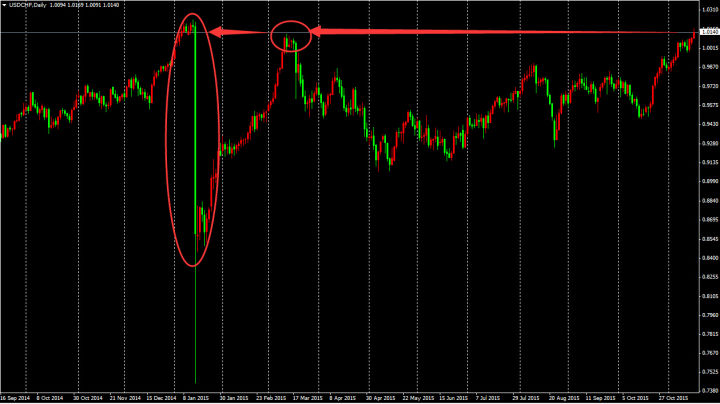
- 4. Although the black swan event is not used commonly, it still has a great impact on quantitative trading. As shown in the chart below, in the case of the black swan event of the foreign exchange Swiss franc, both high and low prices can be seen from the chart. In fact, in the extreme market of the day, the middle price is vacuum, and a large number of stop loss orders cause stampede events. The liquidity is zero, and it is very difficult to deal with, but it can stop loss in the backtest.
Overfitting
Overfitting is a common mistake made by quantitative trading beginners. What is overfitting? To take a simple example, some people use a great deal of exercises to memorize each question in the school exam. He can’t do it if the subject changes a little during the exam. Because he memorized the practice of each question in a very complex way, he did not abstract the general rules.
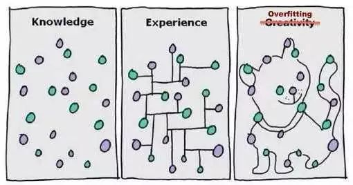
Like the chart above, a model can adapt to data perfectly as long as it is complex enough. This is also true of overfitting in quantitative trading. If your strategy is complex and it has many external parameters, there will always be one or several parameters that can perfectly fit the historical market in the limited historical data backtest.
However, in the future real market, the price change may exceed your strategy limit. In fact, the essence of quantitative trading strategy development is the process of matching local non-random data from a large number of seemingly random data. Therefore, we need to use statistical knowledge to avoid the trap. How do we do it?
The compromise solution is to use intra-sample and extra-sample data. Divide the whole data into two parts, and use the intra-sample as the training set, which is responsible for the data backtest. The extra-sample is used as the test set and is responsible for verification. If there is little historical data, you can also use the cross-test method.
If you find that the data out of the sample performs not well, and you feel that it is too bad to lose the model or you are unwilling to admit that your model is not good, and you continue to optimize the model for the extra-sample data until the extra-sample data also perform well, then you must lose your money in the end.
Survivorship bias
The survivorship bias can be explained by the following examples:
- When standing at the tuyere, pigs will fly.
- People who sell parachutes online are praised, because people with problems with parachutes don’t live anymore.
- The reporter interviewed whether passengers have bought tickets on the bus, because people without tickets can’t get on the bus at all.
- The media advertises that the lottery can be won, because the media will not actively promote people who do not win the lottery.
In the above example, we can find that the information that people usually receive is actually filtered, which makes a large number of data or samples ignored selectively, and the result is that the conclusions based on survivorship bias have deviated from real-time. So in quantitative trading, we also need to focus on whether the results of the backtest are part of luck. In many cases, the results of the backtest may be the best performance in the whole backtest. Pay attention to the following figure:
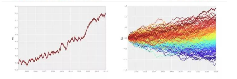
- Left chart (semblance): A very good trading strategy. Without major withdrawal, investors can obtain stable investment returns.
- Right chart (the reality): This is only the best one in 200 random trading backtests.
The picture on the left is a very good trading strategy. The capital curve is good, and there is no significant withdrawal, and stable profit returns can be obtained. But look at the picture on the right. It is only the best one in the hundreds of backtest transactions. On the other hand, when we look at the financial market, there are always more stars and less longevity stars. If the strategy of the traders is consistent with the market situation, then the market every year can create a batch of stars, but it is difficult to see longevity stars who can make steady profits for more than three years in a row.
Cost shock
Unless you are pending an order, you may have a sliding price when trading. On the varieties with active trading, the bid-price and ask-price are usually different in one point. On the varieties with inactive trading, the difference may be greater. Every time you want to take the initiative to close a deal, you need one point difference at least, or even more. However, in the backtest, we do not need to consider the issue of transaction, as long as there is a signal, we can trade, so in order to simulate the real trading environment, we must add one sliding price at least.
Especially for the strategy that is traded more frequently, if the sliding price is not added when the strategy is backtested, the capital curve will always tilt upward, and once the reasonable sliding price is added, it will turn to a loss immediately. In addition, this phenomenon is not only caused by point difference, but also needs to be considered in the real trading environment: network delay, software and hardware systems, server response and other issues.
Strategy capacity
The same strategy will be quite different in efficient and inefficient markets, even the opposite. For example, in inefficient markets such as domestic stock markets, commodity futures, and foreign digital currencies, due to the small base of trading volume, the capacity of high-frequency strategy itself is not very large, and there is no profit space for more people, and even the strategy that was originally profitable has become a loss. But in an efficient foreign exchange market, it can accommodate many different types of high-frequency strategies.
The above are the problems and pitfalls that may occur in the development and use of strategies. For an experienced trading system developer, backtesting is a must. Because it can tell you whether a strategic idea can be verified in historical transactions. But many times, backtesting does not mean that it will be profitable in the future. Because there are too many pitfalls in the backtest, you won’t understand without paying for some lessons. This course can help you avoid many quantitative detours and pitfalls at least.
4.2 Establish the best position management
In “Reminiscences of a stock operator”, there is a very interesting paragraph: the Old Turkey (formerly known as Partridge) who is in the same securities company as the hero Livermore, always makes a big deal. When he was advised to sell after taking profits and buy again after the stock price had retraced. The Old Turkey always intoned: No, you know, this is a bull market!
Even Livermore sighed finally: There is nothing remarkable about the trend. There are always many people who are bullish in the bull market and bearish in the bear market. But they are always good at bargaining with the market, trying to buy at the lowest point and sell at the highest point. Like the Old Turkey, it is those who see the market and hold their positions that really make a great fortune, which is also the most difficult to learn. This not only faces the choice of target and timing, but also faces a more important question: how much position (risk) should we hold (bear)?
All failed traders have one-sided thinking. When trading, greedy people only see profits rather than risks, while timid people only see risks rather than profits. Greedy and timid people forget risks when rising, and forget profits when falling. However, successful traders will consider both risks and returns, that is to say, they will bear several dollars of risk for every dollar they earn. Then the index to measure return and risk is the return risk ratio.
Many people know that the risk is as big as the profit, that is, the return is proportional to the risk. In the view of some people, the relationship between return and risk should be as follows: the horizontal axis is the percentage of risk, and the vertical axis is the percentage of return:
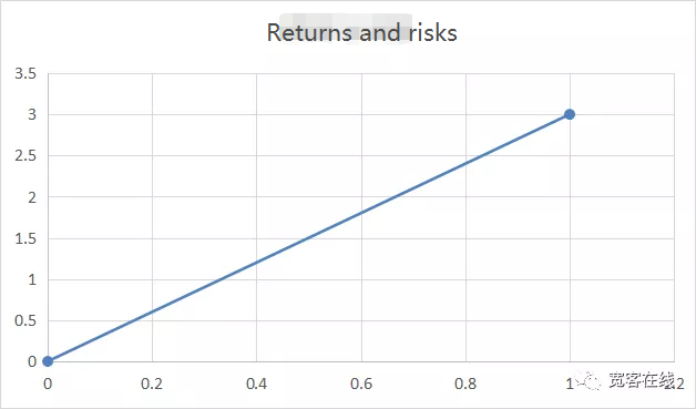
But in the actual transaction, the return and risk are far from being as simple as two points of a line, at least it doesn’t always move linearly. The real risk is the maximum amount of loss that can be taken with the expected return, or what we call the maximum volatility. Although sometimes the maximum floating loss does not always equal the closing loss in terms of the outcome of the trade, the maximum floating loss is real.
From this, we can know that the ratio of return to risk in the figure above is not the real performance. In a real trading environment, the ratio of return to risk should be the same as in the chart below:
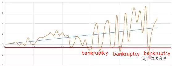
Let’s look at the chart above. The yellow curve shows the fluctuation of net worth at different risks. With the expected returns expanding, the risks are also expanding gradually. If we set bankruptcy at 0.5, that is, the maximum loss reaches 50%, then this is a failed trading strategy. Although the final return of the strategy is positive from the result, it has already gone bankrupt in the middle.
Even if your strategy is a positive one, it will be liquidations under the wrong position management. So from this point of view, how much to buy and sell is more important than when to buy and sell. How to manage the position scientifically has become a fundamental issue in financial transactions. So before trying to solve this problem, let’s see how to bet scientifically in gambling.

Let’s take the coin toss as an example. Suppose that both sides of a coin are equally weighted. If there is a head profit of 2 yuan and a tail loss of 1 yuan, it is obvious that this is a positive expectation game. The winning rate is 50% and a loss of 2. Here comes the question: Now that you have 100 yuan, how can you repeat the bet so that 100 yuan can reach 1 million yuan at the fastest speed.
If we don’t think carefully, we will think that since the return of each bet is 50% * 2-50% * 1, that is, 50%, then in order to achieve the maximum return quickly, we should invest as much capital as possible in each bet. This bet must be 100%.
However, it is obvious that it is unreasonable to invest 100% of the principal in every game of gambling, because as long as you lose the principal once, it will be lost, even if it is very unlikely. Because as long as you gamble enough times, losing money will happen definitely.
Someone may ask, since 100% bet is unreasonable, what about 90% or lower bet? In fact, to solve this problem, we can make an experiment to simulate the gambling game and see how the result of each bet is. As shown in the following chart:
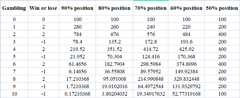
From the chart, we can see that when we gradually reduce the position from 90%, 80%, 70%, 60% and 50%, in the same gamble, the results are completely different. Careful friends may have noticed that with the gradual reduction of the position, the final capital is expanding gradually.
Then some people may ask whether the smaller the bet each time is, the better, such as 10%. It is impossible to calculate every bet proportion. This is the problem to be solved by the famous Kelly Criterion. In statistics, Kelly Criterion can maximize the long-term growth rate of a strategy with positive expectation of repeated bets, and it can calculate the best bet ratio in each bet.
Not only that, assuming that the principal and the bet can be divided endlessly, it is impossible to go bankrupt in any bet by using the Kelly Criterion. Especially in the practical application of financial transactions, it is a position management strategy with both attack and defense. Let’s look at how Kelly Criterion is calculated, and see the following figure:
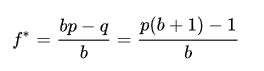
- f is the optimal betting ratio for the available capital;
- b is the odds ratio, which can also be called the profit/loss ratio in trading;
- p is the success rate;
- q is the failure rate.
Then we can calculate the gambling example in this lesson according to the Kelly Criterion. The initial capital of 100 yuan can reach 1 million yuan at the fastest speed by using the betting ratio when the winning ratio is 50% and the odds is 2. Set into the Kelly Criterion, the calculation process is as follows:
(0.5*(2+1) -1)/2=0.25
The winning rate of 50% is 0.5. Multiply the odds by 2 plus 1, then subtract 1, and then divide by 2. The calculation result is 0.25. That is to say, in each bet, using 25% of the principal, you can reach 1 million yuan at the fastest speed. We can simulate manually according to the calculation results to see if it is correct.
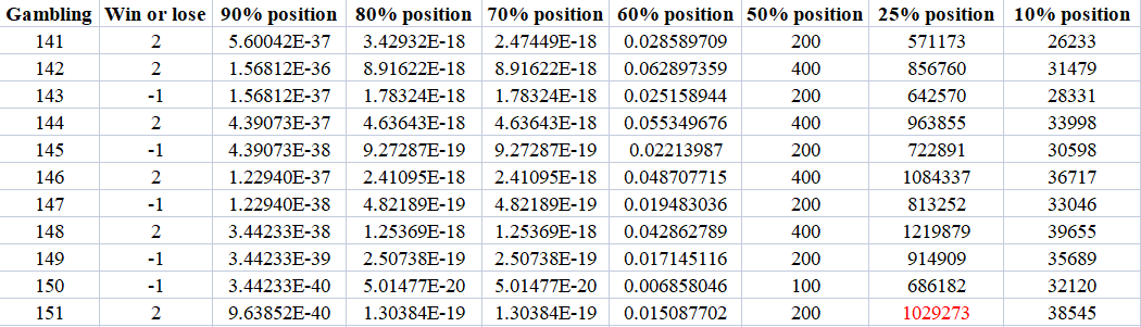
The figure above is the result of manual simulation. Please see the last line. In the same bet, after more than 100 rounds, 25% of the positions reached 1 million yuan first. The result of 90%, 80%, 70% and 60% positions is negative, which shows that even a positive expectation trading strategy will go bankrupt under the wrong position management.
We can also see that 50% of the positions will not lose or win in the end, which is also consistent with the result of the law of large numbers. In order to further illustrate the problem, a position of 10% was also added in the manual simulation. Although the final result was a positive return, the effect was several orders of magnitude worse than that of a position of 25%.
You can see the power of Kelly Criterion. If you choose 10% of the principal position in the actual application, your principal will become more than 30,000 in more than 100 bets. Although the return is large, compared with 25% of the principal position, it is equivalent to no profit. This is the power of knowledge.
If you want to make profits from Kelly Criterion in life, you need to meet the application conditions of Kelly Criterion. There is no doubt that this bet must come from the financial market. Especially in quantitative trading, we can roughly calculate the corresponding winning ratio and odds through historical data backtesting.
Of course, the practical application of Kelly Criterion in financial transactions cannot be so simple, and there are many details to be dealt with, such as the cost of capital in leveraged transactions, the capital and position in real transactions can not be divided wirelessly, and the winning ratio and loss ratio in transactions are changing dynamically, and so on. Whatever, Kelly Criterion shows us how to establish the best position management method.