In the previous article, various methods for calculating mid-price were introduced, and a revised mid-price was proposed. In this article, we will delve deeper into this topic.

Data Required

We need order flow data and depth data for the top ten levels of the order book, collected from live trading with an update frequency of 100ms. For the sake of simplicity, we will not include real-time updates for the bid and ask prices. To reduce the data size, we have kept only 100,000 rows of depth data and separated the tick-by-tick market data into individual columns.

In [1]:

Copy codefrom datetime import date,datetime
import time
import pandas as pd
import numpy as np
import matplotlib.pyplot as plt
import ast
%matplotlib inline

In [2]:

Copy codetick_size = 0.0001

In [3]:

Copy codetrades = pd.read_csv('YGGUSDT_aggTrade.csv',names=['type','event_time', 'agg_trade_id','symbol', 'price', 'quantity', 'first_trade_id', 'last_trade_id',
       'transact_time', 'is_buyer_maker'])

In [4]:

Copy codetrades = trades.groupby(['transact_time','is_buyer_maker']).agg({
    'transact_time':'last',
    'agg_trade_id': 'last',
    'price': 'first',
    'quantity': 'sum',
    'first_trade_id': 'first',
    'last_trade_id': 'last',
    'is_buyer_maker': 'last',
})

In [5]:

Copy codetrades.index = pd.to_datetime(trades['transact_time'], unit='ms')
trades.index.rename('time', inplace=True)
trades['interval'] = trades['transact_time'] - trades['transact_time'].shift()

In [6]:

Copy codedepths = pd.read_csv('YGGUSDT_depth.csv',names=['type','event_time', 'transact_time','symbol', 'u1', 'u2', 'u3', 'bids','asks'])

In [7]:

Copy codedepths = depths.iloc[:100000]

In [8]:

Copy codedepths['bids'] = depths['bids'].apply(ast.literal_eval).copy()
depths['asks'] = depths['asks'].apply(ast.literal_eval).copy()

In [9]:

Copy codedefexpand_bid(bid_data):
    expanded = {}
    for j, (price, quantity) inenumerate(bid_data):
        expanded[f'bid_{j}_price'] = float(price)
        expanded[f'bid_{j}_quantity'] = float(quantity)
    return pd.Series(expanded)
defexpand_ask(ask_data):
    expanded = {}
    for j, (price, quantity) inenumerate(ask_data):
        expanded[f'ask_{j}_price'] = float(price)
        expanded[f'ask_{j}_quantity'] = float(quantity)
    return pd.Series(expanded)
# Apply to each line to get a new df
expanded_df_bid = depths['bids'].apply(expand_bid)
expanded_df_ask = depths['asks'].apply(expand_ask)
# Expansion on the original df
depths = pd.concat([depths, expanded_df_bid, expanded_df_ask], axis=1)

In [10]:

Copy codedepths.index = pd.to_datetime(depths['transact_time'], unit='ms')
depths.index.rename('time', inplace=True);

In [11]:

Copy codetrades = trades[trades['transact_time'] < depths['transact_time'].iloc[-1]]

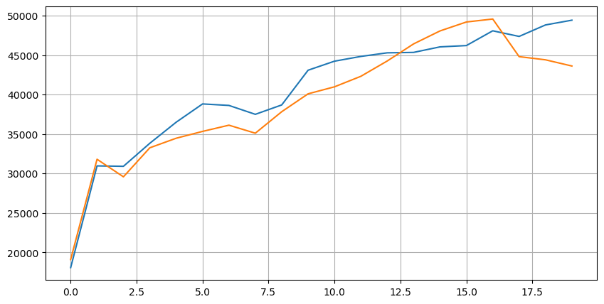
Take a look at the distribution of the market in these 20 levels. It is in line with expectations, with more orders placed the further away from the market price. Additionally, buy orders and sell orders are roughly symmetrical.

In [14]:

Copy codebid_mean_list = []
ask_mean_list = []
for i inrange(20):
    bid_mean_list.append(round(depths[f'bid_{i}_quantity'].mean(),0))
    ask_mean_list.append(round(depths[f'ask_{i}_quantity'].mean(),0))
plt.figure(figsize=(10, 5))
plt.plot(bid_mean_list);
plt.plot(ask_mean_list);
plt.grid(True)

Out[14]:

Merge the depth data with the transaction data to facilitate the evaluation of prediction accuracy. Ensure that the transaction data is later than the depth data. Without considering latency, directly calculate the mean squared error between the predicted value and the actual transaction price. This is used to measure the accuracy of the prediction.

From the results, the error is highest for the average value of the bid and ask prices (mid_price). However, when changed to the weighted mid_price, the error immediately decreases significantly. Further improvement is observed by using the adjusted weighted mid_price. After receiving feedback on using I^3/2 only, it was checked and found that the results were better. Upon reflection, this is likely due to the different frequencies of events. When I is close to -1 and 1, it represents low probability events. In order to correct for these low probability events, the accuracy of predicting high-frequency events is compromised. Therefore, to prioritize high-frequency events, some adjustments were made (these parameters were purely trial-and-error and have limited practical significance in live trading).

The results have improved slightly. As mentioned in the previous article, strategies should rely on more data for prediction. With the availability of more depth and order transaction data, the improvement gained from focusing on the order book is already weak.

In [15]:

Copy codedf = pd.merge_asof(trades, depths, on='transact_time', direction='backward')

In [17]:

Copy codedf['spread'] = round(df['ask_0_price'] - df['bid_0_price'],4)
df['mid_price'] = (df['bid_0_price']+ df['ask_0_price']) / 2
df['I'] = (df['bid_0_quantity'] - df['ask_0_quantity']) / (df['bid_0_quantity'] + df['ask_0_quantity'])
df['weight_mid_price'] = df['mid_price'] + df['spread']*df['I']/2
df['adjust_mid_price'] = df['mid_price'] + df['spread']*(df['I'])*(df['I']**8+1)/4
df['adjust_mid_price_2'] = df['mid_price'] + df['spread']*df['I']*(df['I']**2+1)/4
df['adjust_mid_price_3'] = df['mid_price'] + df['spread']*df['I']**3/2
df['adjust_mid_price_4'] = df['mid_price'] + df['spread']*(df['I']+0.3)*(df['I']**4+0.7)/3.8

In [18]:

Copy codeprint('Mean value     Error in mid_price:', ((df['price']-df['mid_price'])**2).sum())
print('Error of pending order volume weighted mid_price:', ((df['price']-df['weight_mid_price'])**2).sum())
print('The error of the adjusted mid_price:', ((df['price']-df['adjust_mid_price'])**2).sum())
print('The error of the adjusted mid_price_2:', ((df['price']-df['adjust_mid_price_2'])**2).sum())
print('The error of the adjusted mid_price_3:', ((df['price']-df['adjust_mid_price_3'])**2).sum())
print('The error of the adjusted mid_price_4:', ((df['price']-df['adjust_mid_price_4'])**2).sum())

Out[18]:

Mean value Error in mid_price: 0.0048751924999999845
Error of pending order volume weighted mid_price: 0.0048373440193987035
The error of the adjusted mid_price: 0.004803654771638586
The error of the adjusted mid_price_2: 0.004808216498329721
The error of the adjusted mid_price_3: 0.004794984755260528
The error of the adjusted mid_price_4: 0.0047909595497071375

Consider the Second Level of Depth

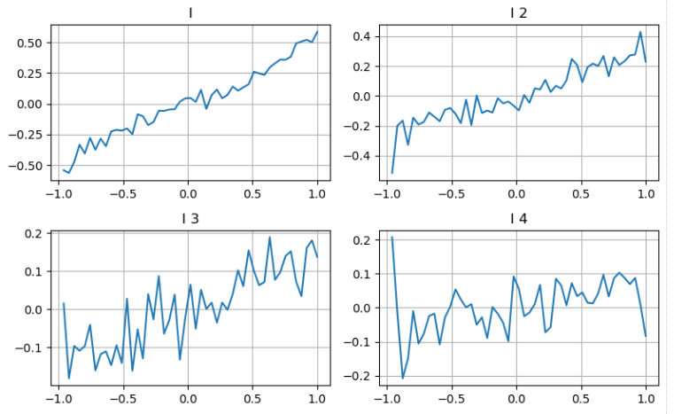
We can follow the approach from the previous article to examine different ranges of a parameter and measure its contribution to the mid_price based on the changes in transaction price. Similar to the first level of depth, as I increases, the transaction price is more likely to increase, indicating a positive contribution from I.

Applying the same approach to the second level of depth, we find that although the effect is slightly smaller than the first level, it is still significant and should not be ignored. The third level of depth also shows a weak contribution, but with less monotonicity. Deeper depths have little reference value.

Based on the different contributions, we assign different weights to these three levels of imbalance parameters. By examining different calculation methods, we observe further reduction in prediction errors.

In [19]:

Copy codebins = np.linspace(-1, 1, 50)
df['change'] = (df['price'].pct_change().shift(-1))/tick_size
df['I_bins'] = pd.cut(df['I'], bins, labels=bins[1:])
df['I_2'] = (df['bid_1_quantity'] - df['ask_1_quantity']) / (df['bid_1_quantity'] + df['ask_1_quantity'])
df['I_2_bins'] = pd.cut(df['I_2'], bins, labels=bins[1:])
df['I_3'] = (df['bid_2_quantity'] - df['ask_2_quantity']) / (df['bid_2_quantity'] + df['ask_2_quantity'])
df['I_3_bins'] = pd.cut(df['I_3'], bins, labels=bins[1:])
df['I_4'] = (df['bid_3_quantity'] - df['ask_3_quantity']) / (df['bid_3_quantity'] + df['ask_3_quantity'])
df['I_4_bins'] = pd.cut(df['I_4'], bins, labels=bins[1:])
fig, axes = plt.subplots(nrows=2, ncols=2, figsize=(8, 5))


axes[0][0].plot(df.groupby('I_bins')['change'].mean())
axes[0][0].set_title('I')
axes[0][0].grid(True)

axes[0][1].plot(df.groupby('I_2_bins')['change'].mean())
axes[0][1].set_title('I 2')
axes[0][1].grid(True)

axes[1][0].plot(df.groupby('I_3_bins')['change'].mean())
axes[1][0].set_title('I 3')
axes[1][0].grid(True)

axes[1][1].plot(df.groupby('I_4_bins')['change'].mean())
axes[1][1].set_title('I 4')
axes[1][1].grid(True)
plt.tight_layout();

Out[19]:

In [20]:

Copy codedf['adjust_mid_price_4'] = df['mid_price'] + df['spread']*(df['I']+0.3)*(df['I']**4+0.7)/3.8
df['adjust_mid_price_5'] = df['mid_price'] + df['spread']*(0.7*df['I']+0.3*df['I_2'])/2
df['adjust_mid_price_6'] = df['mid_price'] + df['spread']*(0.7*df['I']+0.3*df['I_2'])**3/2
df['adjust_mid_price_7'] = df['mid_price'] + df['spread']*(0.7*df['I']+0.3*df['I_2']+0.3)*((0.7*df['I']+0.3*df['I_2'])**4+0.7)/3.8
df['adjust_mid_price_8'] = df['mid_price'] + df['spread']*(0.7*df['I']+0.2*df['I_2']+0.1*df['I_3']+0.3)*((0.7*df['I']+0.3*df['I_2']+0.1*df['I_3'])**4+0.7)/3.8

In [21]:

Copy codeprint('The error of the adjusted mid_price_4:', ((df['price']-df['adjust_mid_price_4'])**2).sum())
print('The error of the adjusted mid_price_5:', ((df['price']-df['adjust_mid_price_5'])**2).sum())
print('The error of the adjusted mid_price_6:', ((df['price']-df['adjust_mid_price_6'])**2).sum())
print('The error of the adjusted mid_price_7:', ((df['price']-df['adjust_mid_price_7'])**2).sum())
print('The error of the adjusted mid_price_8:', ((df['price']-df['adjust_mid_price_8'])**2).sum())

Out[21]:

The error of the adjusted mid_price_4: 0.0047909595497071375
The error of the adjusted mid_price_5: 0.0047884350488318714
The error of the adjusted mid_price_6: 0.0047778319053133735
The error of the adjusted mid_price_7: 0.004773578540592192
The error of the adjusted mid_price_8: 0.004771415189297518

Considering the Transaction Data

Transaction data directly reflects the extent of long and short positions. After all, transactions involve real money, while placing orders has much lower costs and can even involve intentional deception. Therefore, when predicting the mid_price, strategies should focus on the transaction data.

In terms of form, we can define the imbalance of the average order arrival quantity as VI, with Vb and Vs representing the average quantity of buy and sell orders within a unit time interval, respectively.

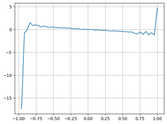
The results show that the arrival quantity in a short period of time has the most significant impact on price change prediction. When VI is between 0.1 and 0.9, it is negatively correlated with price, while outside this range, it is positively correlated with price. This suggests that when the market is not extreme and mainly oscillates, the price tends to revert to the mean. However, in extreme market conditions, such as when there are a large number of buy orders overwhelming sell orders, a trend emerges. Even without considering these low probability scenarios, assuming a negative linear relationship between the trend and VI significantly reduces the prediction error of the mid_price. The coefficient "a" represents the weight of this relationship in the equation.

In [22]:

Copy codealpha=0.1

In [23]:

Copy codedf['avg_buy_interval'] = None
df['avg_sell_interval'] = None
df.loc[df['is_buyer_maker'] == True, 'avg_buy_interval'] = df[df['is_buyer_maker'] == True]['transact_time'].diff().ewm(alpha=alpha).mean()
df.loc[df['is_buyer_maker'] == False, 'avg_sell_interval'] = df[df['is_buyer_maker'] == False]['transact_time'].diff().ewm(alpha=alpha).mean()

In [24]:

Copy codedf['avg_buy_quantity'] = None
df['avg_sell_quantity'] = None
df.loc[df['is_buyer_maker'] == True, 'avg_buy_quantity'] = df[df['is_buyer_maker'] == True]['quantity'].ewm(alpha=alpha).mean()
df.loc[df['is_buyer_maker'] == False, 'avg_sell_quantity'] = df[df['is_buyer_maker'] == False]['quantity'].ewm(alpha=alpha).mean()

In [25]:

Copy codedf['avg_buy_quantity'] = df['avg_buy_quantity'].fillna(method='ffill')
df['avg_sell_quantity'] = df['avg_sell_quantity'].fillna(method='ffill')
df['avg_buy_interval'] = df['avg_buy_interval'].fillna(method='ffill')
df['avg_sell_interval'] = df['avg_sell_interval'].fillna(method='ffill')

df['avg_buy_rate'] = 1000 / df['avg_buy_interval']
df['avg_sell_rate'] =1000 / df['avg_sell_interval']

df['avg_buy_volume'] = df['avg_buy_rate']*df['avg_buy_quantity']
df['avg_sell_volume'] = df['avg_sell_rate']*df['avg_sell_quantity']

In [26]:

Copy codedf['I'] = (df['bid_0_quantity']- df['ask_0_quantity']) / (df['bid_0_quantity'] + df['ask_0_quantity'])
df['OI'] = (df['avg_buy_rate']-df['avg_sell_rate']) / (df['avg_buy_rate'] + df['avg_sell_rate'])
df['QI'] = (df['avg_buy_quantity']-df['avg_sell_quantity']) / (df['avg_buy_quantity'] + df['avg_sell_quantity'])
df['VI'] = (df['avg_buy_volume']-df['avg_sell_volume']) / (df['avg_buy_volume'] + df['avg_sell_volume'])

In [27]:

Copy codebins = np.linspace(-1, 1, 50)
df['VI_bins'] = pd.cut(df['VI'], bins, labels=bins[1:])
plt.plot(df.groupby('VI_bins')['change'].mean());
plt.grid(True)

Out[27]:

In [28]:

Copy codedf['adjust_mid_price'] = df['mid_price'] + df['spread']*df['I']/2
df['adjust_mid_price_9'] = df['mid_price'] + df['spread']*(-df['OI'])*2
df['adjust_mid_price_10'] = df['mid_price'] + df['spread']*(-df['VI'])*1.4

In [29]:

Copy codeprint('The error of the adjusted mid_price:', ((df['price']-df['adjust_mid_price'])**2).sum())
print('The error of the adjusted mid_price_9:', ((df['price']-df['adjust_mid_price_9'])**2).sum())
print('The error of the adjusted mid_price_10:', ((df['price']-df['adjust_mid_price_10'])**2).sum())

Out[29]:

The error of the adjusted mid_price: 0.0048373440193987035
The error of the adjusted mid_price_9: 0.004629586542840461
The error of the adjusted mid_price_10: 0.004401790287167206

The Comprehensive Mid-price

Considering that both order book imbalance and transaction data are helpful for predicting the mid_price, we can combine these two parameters together. The assignment of weights in this case is arbitrary and does not take into account boundary conditions. In extreme cases, the predicted mid_price may not fall between the bid and ask prices. However, as long as the prediction error can be reduced, these details are not of great concern.

In the end, the prediction error is reduced from 0.00487 to 0.0043. At this point, we will not delve further into the topic. There are still many aspects to explore when it comes to predicting the mid_price, as it is essentially predicting the price itself. Everyone is encouraged to try their own approaches and techniques.

In [30]:

Copy code#Note that the VI needs to be delayed by one to use
df['CI'] = -1.5*df['VI'].shift()+0.7*(0.7*df['I']+0.2*df['I_2']+0.1*df['I_3'])**3

In [31]:

Copy codedf['adjust_mid_price_11'] = df['mid_price'] + df['spread']*(df['CI'])
print('The error of the adjusted mid_price_11:', ((df['price']-df['adjust_mid_price_11'])**2).sum())

Out[31]:

The error of the adjusted mid_price_11: 0.0043001941412563575

Summary

The article combines depth data and transaction data to further improve the calculation method of the mid-price. It provides a method to measure accuracy and improves the accuracy of price change prediction. Overall, the parameters are not rigorous and are for reference only. With a more accurate mid-price, the next step is to conduct backtesting using the mid-price in practical applications. This part of the content is extensive, so updates will be paused for a period of time.