
The ANT spread between Binance and trade.xyz has attracted plenty of discussion over the past few days.
Both Binance and trade.xyz list a pre-IPO contract linked to Anthropic. In the November 2–5 sample discussed here, converting the quotes to a per-share price using an assumed 12.7 billion shares consistently made Binance the more expensive venue. If the final share count and the exchanges’ rebasing rules match that assumption, the two quotes could move onto a common share-count basis, allowing us to assess convergence on that basis.
With the quantities on both venues matched using this assumption, the position is short Binance and long xyz, waiting for the spread to narrow.
During these live trading sessions, the spread narrowed sharply several times, then widened again. Holding the position throughout would have meant giving back the unrealized gains along the way. I split the position into several paired tranches, reducing one when the spread narrowed and adding it back after the spread widened, to see whether those swings could produce a return.
1. What the Spread Did Over Those Few Days
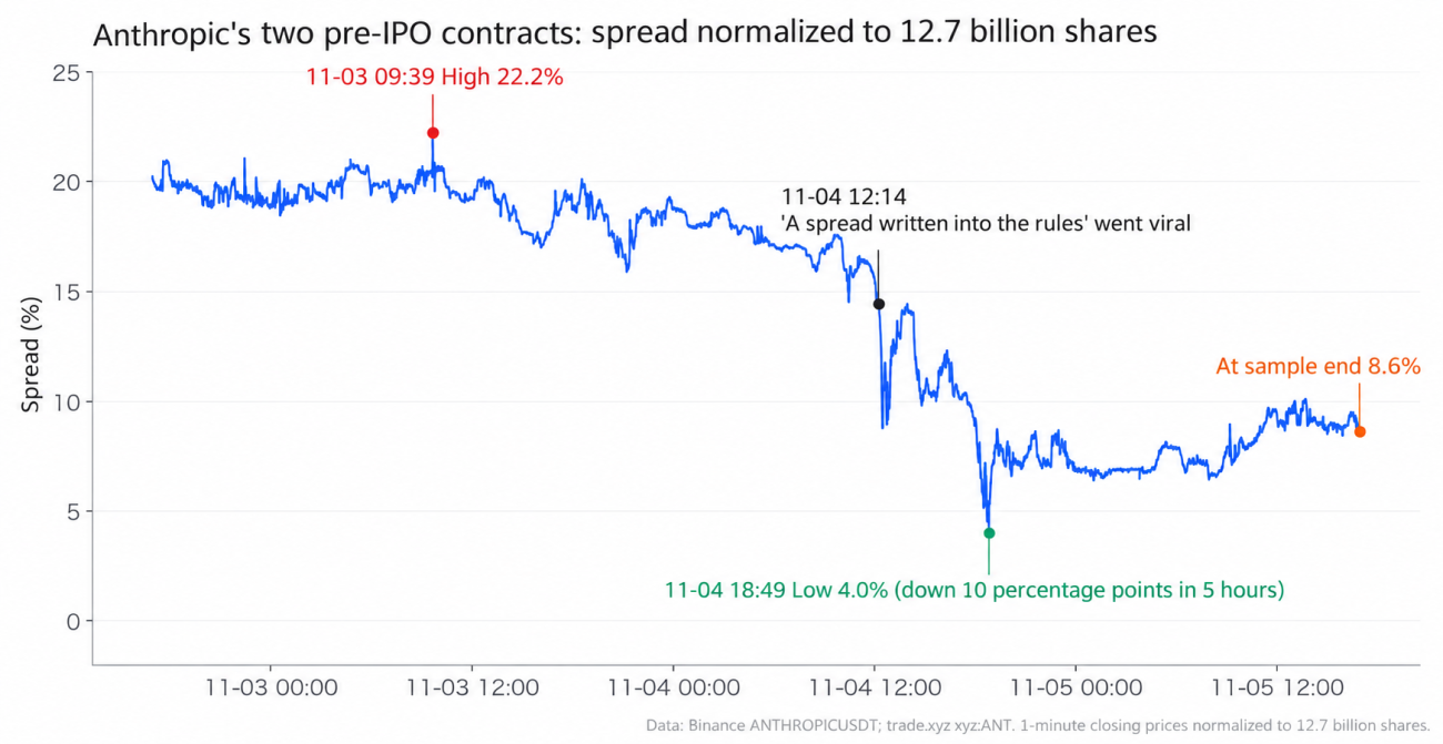
On November 2 and 3, the spread hovered around 20%, reaching a high of 22.2% on the morning of the 3rd.
Around noon on the 4th, Silicon Bird (@limxn6) published a post about an arbitrage spread “written into the rules.” It broke down the prospectus item by item and estimated that the exchanges would rebase using roughly 12.7 billion shares. The post drew more than 60,000 views.
That afternoon, the spread fell from 14% to 4% in five hours.
The decline did not last. The spread rebounded to 7% that evening and was back above 9% by the afternoon of November 5.
If you had jumped in at 4% late on the 4th, thinking convergence had begun, the spread would have moved 590 bps against you over the next day.
2. What Else Matters When Holding This Pair
The share count used for conversion was still uncertain.
The same prospectus supported two different ways of counting:
- 12.7 billion: the estimated shares outstanding at the IPO. Exchanges have used an outstanding-share basis for rebasing, including for SpaceX.
- 16.6–16.9 billion: a fully diluted estimate, including options, unvested RSUs, and the portion of Amazon’s convertible notes above the ownership cap. This estimate was derived from the prospectus. Entropy uses a fully diluted share-count basis after an IPO.
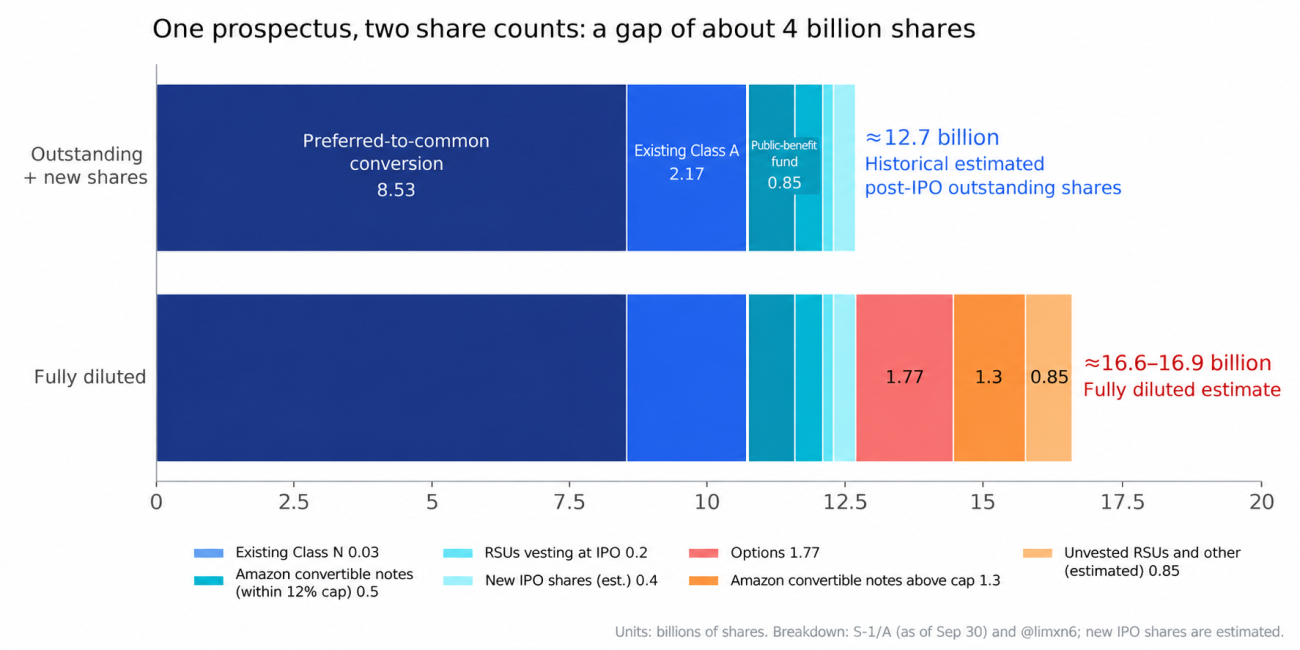
The two estimates differ by roughly 4 billion shares, which changes the relative prices after conversion:
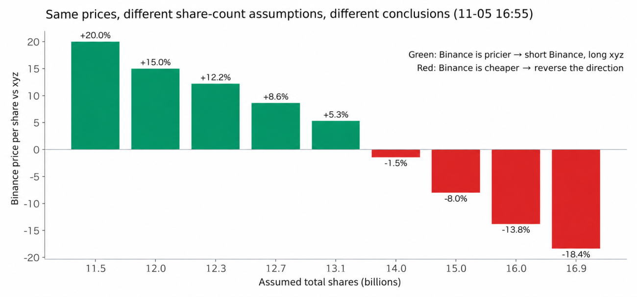
Using prices from the same moment, Binance was 8.6% more expensive under a 12.7 billion-share assumption. At 14 billion shares, Binance was instead 1.5% cheaper.
The calculations in this historical analysis use 12.7 billion shares. If that number changes, both the relative prices and the matched quantities need to be recalculated. A grid cannot resolve this uncertainty.
Margin must be monitored separately on each venue.
The two legs sit on different exchanges, with separate margin accounts. When the spread widens, the combined position may show only a small loss while one leg is already under pressure. Unrealized gains on the other venue do not automatically move across to support it. Insufficient margin could force a reduction before the trade has time to play out.
Both legs tie up capital while the position is open.
At the time, trade.xyz displayed November 20 as the expected IPO date. If the plan were simply to wait for the final convergence, capital would remain committed on both venues throughout the holding period. The spread might swing up and down dozens of times along the way, and the position would just ride through them.
3. Splitting the Position and Trading It in Tranches
A closer look at the spread over those few days showed that:
- The median spread range within a 10-minute window was 34 bps.
- Half of the observations were between 21 and 63 bps.
- Taker fees for the four fills needed to open and close both legs totaled approximately 10 bps.
Moves of several dozen basis points were common in this sample. But 10 bps covered only commissions at the fee rates used at the time. Bid-ask spreads, slippage, the timing difference between the two legs, and funding still needed to be accounted for separately.
Execution matters too. The 34 bps figure was an observed range, not an amount a strategy could necessarily capture. After bid-ask spreads, execution differences, and fees, the remaining room would be smaller.
The direction of the pair stays the same: short Binance and long xyz. The position is split into tranches, each reduced and replenished when its conditions are met.
When the spread narrows enough to meet a tranche’s reduction conditions, both legs of that tranche are closed. If the spread widens again and conditions are suitable, a paired tranche is reopened in the same direction. Its new execution level is recorded, ready for the next narrowing move.
Here is a simulation of the two approaches using the same historical market data and the same starting position:
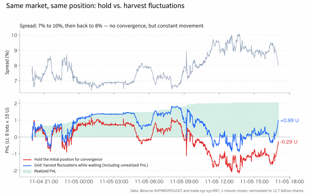
From 20:00 on November 4 to 17:00 on November 5, the spread moved from 7% to 10% and then back to 8%. It did not converge, but it kept moving.
- Hold throughout: −0.29 U, after spending a considerable stretch near −2 U.
- Trade the swings while waiting: +0.99 U including unrealized P&L, with 2.05 U realized in the simulation.
Several rounds of trading were completed in this simulation even though final convergence had not yet occurred. However, realized results and the unrealized P&L on the remaining position must be considered together. Looking only at the gains already realized would give an incomplete picture.
4. Using Two Timeframes for Position Sizing and Grid Spacing
The first version divided the distance from the entry spread to the take-profit line into equal steps when the position was opened. Each step was 115 bps, and that spacing stayed fixed.
The spread then swung back and forth for more than three hours, moving 40–50 bps at a time. Not a single tranche was sold, while the position showed an unrealized loss of 2.1 U. The strategy simply watched those swings go by.
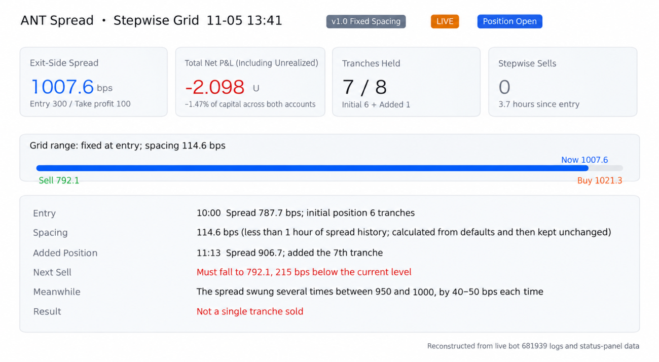
The 115 bps spacing did not adjust to the subsequent volatility, so several 40–50 bps swings never reached the next level. The revised approach uses two timeframes: the longer timeframe determines the initial position for each cycle, and the shorter timeframe calculates the trading intervals while the position is open.
First, use the longer timeframe to determine the initial position.
By default, the strategy examines the past 24 hours of spread data. The area between the 10th and 90th percentiles indicates where the spread has mainly been trading. The most extreme observations at either end are excluded from the normal range, but that does not mean the spread cannot move beyond it.
The initial position depends on three things together: where the current spread sits within that range, the actual available balance on each venue, and the room for further narrowing after allowing for costs and budgeted funding.
A higher position within the range can support a larger initial position. Near the lower edge, there may not be enough room for another grid tranche even if cash remains available. When capacity allows, some allocation is reserved for later additions—approximately one quarter by default. If capacity is sufficient for only one tranche, there is no room to set aside another full tranche.
At startup, the strategy first loads closed historical bars matched to the same minute on both venues. If the history is insufficient, contains too many gaps, or is stale, it waits. It does not open a position using an arbitrary default range.
Second, use the shorter timeframe to calculate trading intervals.
By default, the strategy looks at the past 30 minutes and again uses the central trading range to estimate the spread’s amplitude. Under the current default settings, the intervals for both reductions and additions are approximately one third of that range, subject to a cost floor: the larger of the two values is used.
The reduction and addition coefficients can be configured separately, although their defaults are the same. The longer timeframe determines position size only at the start of a cycle. During the cycle, the shorter timeframe updates the grid spacing.
Immediately after a tranche is reduced, the next refill uses the current reduction interval, measured from the last actual execution spread. Once the tranche is reopened, the reference point is updated again for the next action.
Third, update the execution reference while retaining each tranche’s cost basis.
Each tranche retains the average entry price of both legs. Subsequent trades update the grid reference point, while the original entry costs remain available for checking that tranche’s reduction conditions.
Before reducing a tranche, the strategy checks both the previous execution level and that tranche’s entry costs. It then estimates the net result of closing it using the actual average prices and quantities of both legs, the configured fees, and the funding budget accumulated over that tranche’s holding period. A normal grid reduction is allowed only if the estimated result meets the minimum net-profit requirement.
Even if the initial tranches have similar entry costs, they are handled one at a time. Selling one updates the reference point, so the spread must narrow further before the next one can be sold. Touching a single level does not trigger the sale of the entire initial position.
Fourth, include execution costs in the minimum grid spacing.
The revised minimum spacing includes more than the fees for four fills. It also allows for slippage on both legs and a minimum net-profit margin.
With the current default settings, the fee budget is 10 bps, the combined slippage budget for both legs is another 10 bps, and the minimum net-profit allowance is 5 bps. That produces a minimum spacing of 25 bps. These are configured budgets, not a claim that every trade incurs exactly those costs.
When volatility decreases, the calculated spacing can tighten; when volatility increases, it widens. The earlier rules that compressed spacing as waiting time grew, or widened it based on recent trade results, have been removed. If there is not enough room, the strategy lets that small swing pass.
Fifth, recheck trading conditions before every addition.
Before adding a tranche, the strategy rechecks both balances, effective leverage, the cycle’s total capacity, and the remaining profit potential. It also checks order-book depth and the current grid range.
If the spread suddenly jumps above the grid’s current upper boundary, the strategy waits for the range to update instead of chasing the move. It also holds off on the next order if quotes from the two venues are out of sync, account data is not ready, or the outcome of the preceding order remains unresolved.
Sixth, settle a completed cycle and plan the next one.
All initial tranches participate in the grid; no fixed portion is held back solely for final convergence. Once the final tranche has been closed, both legs are flat, and no orders remain unresolved, the cycle is settled.
The strategy then reassesses the longer-term range, current balances, and available room to plan the next cycle. It does not carry forward the previous cycle’s cost basis, reference points, or initial tranche count. It no longer waits for a rebound using an old reference point, and the spread does not have to narrow to 1% for a cycle to end. By default, there is no additional waiting period between cycles, although the new plan still has to pass the ongoing confirmation checks.
An additional spread protection threshold can be configured separately; it is disabled by default. If contract units or rules change, the strategy first stops opening new positions and adding to existing ones. Conversion assumptions and actual holdings must then be checked before deciding what to do next. An announcement alone is not treated as an automatic instruction to close everything.
Here are the execution points for fixed spacing and volatility-adjusted spacing over the same historical period:
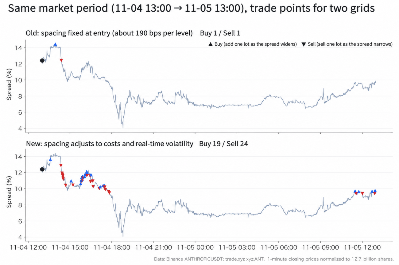
The fixed grid made 1 buy and 1 sell. The dynamic grid made 19 buys and 24 sells.
5. Live Trading on the Afternoon of November 5
Looking back at that afternoon’s session, a paired position was opened at 15:31. Each account held roughly 70 U, and the position was split into 8 tranches of 15 U each.
The entry spread at 15:31 was 888 bps. Over the next hour and a half, the spread fluctuated between 850 and 950 bps, and the strategy made six sales.
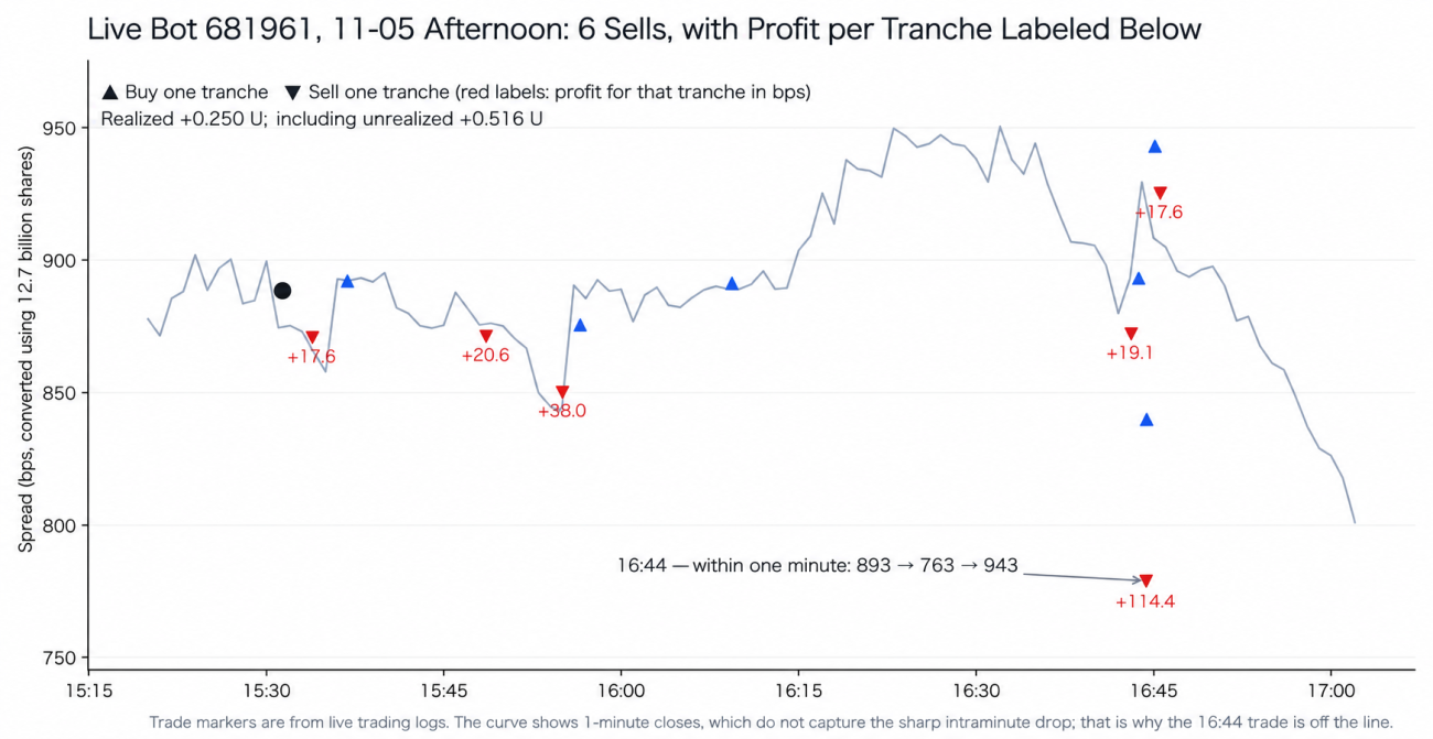
Around 16:44, there were four consecutive reductions and additions.
Within a single minute, the spread dropped from 893 to 763 bps, then rebounded to 943 bps. That spike is not visible in a line plotted from one-minute closes.
The grid sold one tranche at 778.8 bps, capturing 114 bps of spread movement—more than the previous four sales combined. As the spread rebounded, it reopened a tranche at 839.7 bps, added another at 942.9 bps, and sold again when the spread fell back to 925 bps.
With fixed spacing, the next sell level for that cycle would have been 757 bps. The spike bottomed at 763 bps before rebounding, missing the level by 6 bps. No tranche would have been sold.
6. What Still Needs Monitoring
- Directional risk remains. The grid does not change the 12.7 billion-share assumption underlying this historical trade. The S-1/A amendment filed on November 10, 2026 already includes an indicative IPO price range and updated capitalization information. Any continued trading must recheck the latest filings and the exchanges’ conversion rules. If the underlying assumption no longer holds, stop and reassess.
- Monitor margin separately on both venues. A profitable combined position does not mean both accounts are safe. Keep leverage modest. If either leg approaches its margin limit, reduce both legs together.
- The number of tranches depends on actual conditions on both venues. Available balances, minimum order sizes, and the quantities needed to match the two legs all constrain the tranche count. The initial position in each cycle also depends on the longer-term range and remaining profit potential. It is not always a full eight-tranche position.
- Commissions are only part of the cost. The minimum grid spacing must also allow for slippage on both legs and a minimum net-profit margin, while funding over the holding period must be considered. The strategy’s cycle-level net result is still an estimate based on configured fee rates and funding budgets. The exchanges’ actual settlement figures are what ultimately count.
- Keep monitoring the contract window and conversion rules. An expected date is not a final execution schedule. If units or rules change, the relative prices, hedge quantities, and existing positions all need to be checked again.
While waiting for the final rules, holding the position unchanged is not the only option. The longer timeframe determines how each cycle begins; the shorter timeframe handles the swings while the position is open. Once a cycle ends, the next one is planned around the new conditions.
The next things I want to track are the pressure on positions when the spread keeps widening, and whether actual execution costs leave enough room for these small trades to generate a net return.
The live trading shown here is mainly intended to explore whether this approach is workable. Both the capital involved and the observation period are limited. At larger sizes, order-book depth, market impact, and execution differences between the two legs become more important. You can also build on this approach with AI assistance to improve liquidity constraints, order splitting, and execution methods, then test those changes against your own capital size and trading conditions.
DYOR. This article is a record of my own trading, not investment advice.