
At 11:30 on August 30, Binance listed the USDT-margined perpetual contract for 牛来, whose contract symbol is literally the Chinese 牛来USDT. The coin comes from a Chinese animated film that two people spent five years making and that went viral partly because of its rough-looking visuals. On top of that, 牛来 sounds like “the bull market is coming,” and that is how the meme took off. On its first day of trading, its 24-hour amplitude reached 57.4%, it rose 28.7% in a single day, and its minute-based realized volatility reached 95.7 basis points. I compared it cross-sectionally against 612 perpetual contracts across the entire market, and it ranked first in both the depth and frequency of lower wicks.
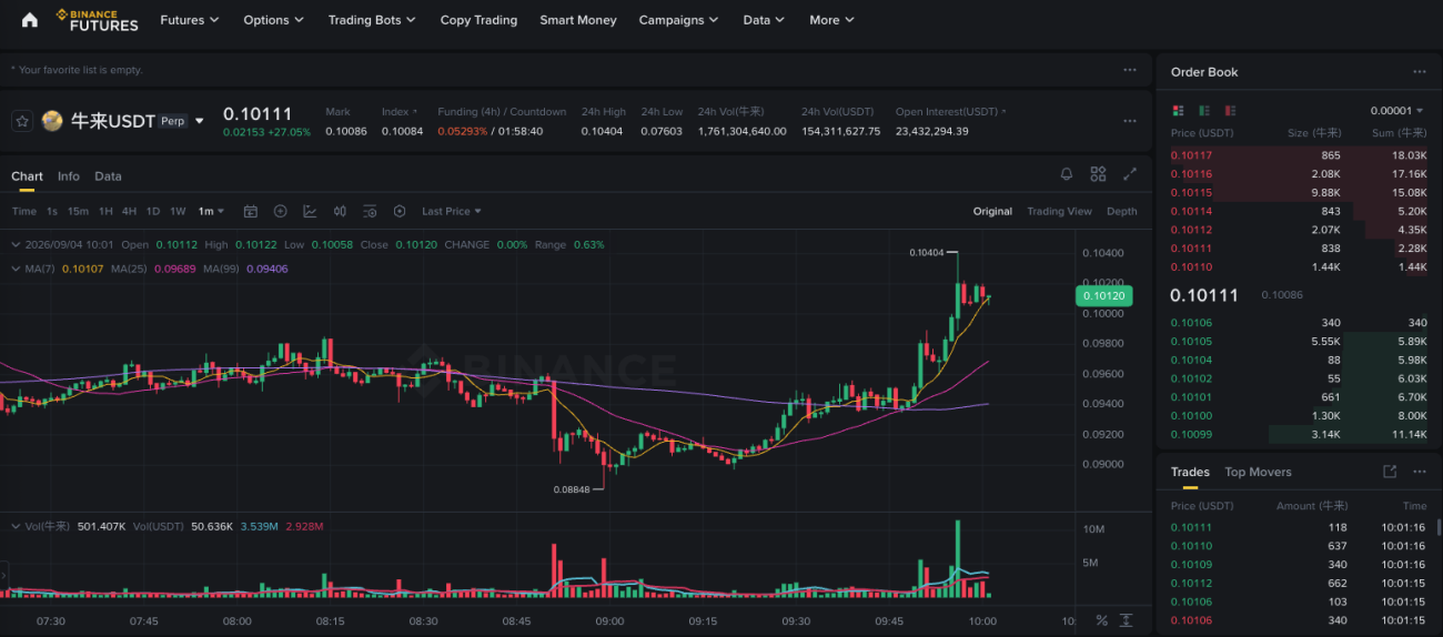
That is also where the problem starts. With volatility like this, if you chase the long side, you do not know whether you are buying at the top; if you short it, one wick can blow you up. I was afraid of both the highs and the lows, so I did not dare take either side. But with roughly $400 million in daily turnover sitting there, I also did not want to just watch from the sidelines.
On this type of coin, I first tried several of the most intuitive approaches: placing low bids to catch wicks, running a two-sided grid, and arbitraging around funding settlements. None of them worked. Looking back, the reason for failure was the same in every case: they were all betting that “if price falls, it will bounce back.” Catching wicks bets on mean reversion after a deep wick; grids bet on price oscillating within a range; funding-rate sniping bets on a post-settlement price reversal. But the data gave a very consistent answer: the deep-wick reversion rate for 牛来 was only 0.31; shallow pullbacks had a reversion rate of 1.65, but the order-book queue made them practically impossible to fill; and in a 139-day grid sample, sideways and rising windows were almost always profitable, while large down-move windows had a win rate of only 8%.
High-volatility meme perpetuals are momentum assets, not mean-reverting assets. Once I understood that, only one direction remained: do not fight them; move with them.

The Strong Stay Strong, and How to Define “Strong”
The simplest form of a trend-following strategy is to buy the assets that have risen the most and sell the assets that have fallen the most. But looking only at returns has an obvious flaw: return is the result, not the cause. A coin may be up 20% because sustained new capital is pushing it higher, or it may be up because a few short-covering trades caused a temporary squeeze. The subsequent paths of those two situations can be completely different, even though the candles look identical.
So I added a second dimension: the funding rate.
The funding rate of a perpetual contract is essentially a mechanism for balancing the holding costs between longs and shorts. When the funding rate is pushed higher, it means a large number of traders are willing to keep paying to hold long positions. That is different from simply saying “the price went up.” A large order can push price higher, but the funding rate reflects the structure of open positions and therefore represents real willingness to pay to maintain that exposure.
Price momentum tells you, “it went up.” The funding rate tells you, “someone is willing to pay to stay in this direction.” Combine these two dimensions into a composite momentum score, go long the highest-scoring group and short the lowest-scoring group, with equal notional amounts on both sides. If the whole sector rises or falls together, the long and short legs offset each other. The return comes only from the relative performance between “the strongest group” and “the weakest group.” This directly avoids the original dilemma: you do not need to predict whether 牛来 will rise or fall; you only need to judge whether it is stronger or weaker than the other speculative coins.

How Much Weight Should Each of the Two Factors Get?
At first, I used fixed coefficients: 1.0 for price momentum and 0.6 for funding. Once I ran it, I immediately felt something was wrong. Those two numbers were chosen by intuition and had no real basis. Why 0.6 instead of 0.4?
The bigger problem is that even if I find the coefficients that are optimal right now, they may not remain stable. During testing I observed something interesting: for the very same funding-rate factor, changing the universe from 44 contracts to 35, or changing the time window from 41 days to 31 days, could flip the sign of its performance. If a factor can change sign as market conditions change, using a fixed weight effectively welds the characteristics of one historical regime permanently into the strategy.
So I changed the system to let the data decide. The method is rolling cross-sectional regression: at each period, use all candidate contracts available at that time to run a cross-sectional OLS regression of the next-period realized return on the z-scores of the two factors.
// Single-period cross-sectional OLS:// fwd = a + b1*z(momentum) + b2*z(funding)functioncrossSectionOLS(zm, zf, fwd) {
    var n = fwd.length; if (n < 10) returnnull;
    var A = [[0,0,0],[0,0,0],[0,0,0]], b = [0,0,0];
    for (var i = 0; i < n; i++) {
        var x = [1, zm[i], zf[i]];
        for (var r = 0; r < 3; r++) {
            b[r] += x[r] * fwd[i];
            for (var c = 0; c < 3; c++) A[r][c] += x[r] * x[c];
        }
    }
    returnsolve3(A, b);
}
Run this period by period over the past 120 periods (one period every four hours, or about 20 days), obtain a time series of coefficients for both factors, and then take the time-series mean. This is the Fama-MacBeth approach. The mean gives you the weight; the standard deviation gives you the significance.
The key question is how to use that significance. A coefficient mean can be large, but if it jumps around wildly over time, then the factor behaves very differently in different periods and should not receive a high weight. So the coefficient is shrunk using its t-statistic:
functionshrink(r) {
    var k = Math.min(1, Math.abs(r.t) / T_SHRINK);   // Full weight when |t|>=2; otherwise shrink proportionallyreturn r.m * k;
}
var w1 = shrink(r1), w2 = shrink(r2);
var scale = Math.abs(w1) + Math.abs(w2);
w1 = w1 / scale;  w2 = w2 / scale;                  // Normalize so |w1|+|w2|=1
This has three benefits. An insignificant factor is automatically downweighted, so I do not need to decide manually how much weight each one deserves. The sign is determined by the data: if, during some period, the correct use of the funding factor is contrarian, the regression will produce a negative coefficient and the strategy will follow it instead of stubbornly keeping the positive sign I originally wrote down. And once the weights are normalized, total exposure is unaffected; only the relative influence of the two factors changes.
The model is refit every 12 hours. The dashboard directly displays the β and t-values of the two factors, so you can see where the current weights come from. If one day the t-value of the funding factor drops to 0.3, you will see its weight automatically shrink close to the lower bound instead of remaining hidden from view.
A Pitfall That Must Be Fixed: The Time Basis of Funding Rates
This is something I ran into during implementation, and its impact is large enough to deserve its own section.
Different Binance contracts have different funding settlement intervals. Querying the fundingInfo endpoint, among the 768 contracts with records across the whole market, 440 settle every four hours, 324 every eight hours, and another four every one hour. 牛来 itself settles every four hours.
The problem is that a contract settling every four hours at a funding rate of five basis points and a contract settling every eight hours at five basis points display the same nominal number, but the true holding cost differs by a factor of two. The former charges six times per day; the latter only three times.
If raw funding rates are used directly for cross-sectional ranking, you are effectively comparing numbers with different units. This systematically pushes four-hour contracts lower and eight-hour contracts higher, even though more than half of the universe consists of four-hour contracts. The selected long and short legs become distorted.
The fix is simple, but it cannot be skipped:
// Pull each contract's settlement intervalvar fi = api('fundingInfo');
for (var i = 0; i < fi.length; i++)
    _ivh[fi[i].symbol] = parseInt(fi[i].fundingIntervalHours || 8);

// ★ Normalize to an 8-hour basis before ranking
c.fund8 = c.fr * (8.0 / ivh(c.bin));
Risk Parity: Make Each Coin Contribute the Same Amount of Risk
Volatility differs enormously across a meme-coin universe. Within the same candidate set, four-hour volatility can range from 15 basis points to 200 basis points. If notional amounts are allocated equally, the two or three most volatile coins can contribute more than 80% of the portfolio’s risk while the rest are effectively irrelevant. On paper you may hold ten coins, but in practice you are betting on only two of them.
So within each leg, weights are assigned inversely to volatility:
functionriskParity(g) {
    var iv = [], z = 0;
    for (var i = 0; i < g.length; i++) { var x = 1 / Math.max(5, g[i].sigma); iv.push(x); z += x; }
    var w = []; for (var j = 0; j < g.length; j++) w.push(iv[j] / z);
    return w;
}
Among all the improvements I tried, this was the only one that improved all three metrics across the full sample at the same time: the median increased from 36.5 basis points to 68.0, the win rate rose from 53% to 57%, and the worst single result narrowed from -2021 to -1422. This is not parameter fitting; it is structural. Once risk is distributed more evenly, portfolio performance is no longer determined by the luck of one or two coins.
At the portfolio level, another layer of target-volatility scaling is added. First estimate the volatility level of the current candidate portfolio. If it is above the target, reduce total exposure proportionally; if it is below the target, keep exposure at the cap:
var pv = 0;
for (var a = 0; a < L.length; a++) pv += wl[a] * L[a].sigma;
for (var b = 0; b < Sh.length; b++) pv += ws[b] * Sh[b].sigma;
pv = pv / 2 * 0.6 / 1e4 * 100;                         // Residual volatility estimate after long/short hedgingvar scale = pv > 0 ? Math.min(1, TARGET_VOL_PCT / pv) : 1;
var gross = GROSS_MAX_USDT * scale;
The point of this is to make the return distribution more predictable. Meme-coin markets can be extremely quiet at times and explode all at once at others. Fixed notional exposure means your true risk can drift by several multiples depending on market conditions. Target-volatility scaling smooths that drift, at the cost of automatically reducing positions when the market is at its most violent — which is exactly when they should be reduced.

Unified Account: Unrealized Losses on Long and Short Legs Offset Each Other
This is one of the easiest things to overlook in live trading for this kind of strategy, yet it has one of the largest impacts on survival.
Suppose you hold ten longs and ten shorts. Under isolated margin, maintenance margin is calculated independently for each leg. Any single leg that reaches its liquidation threshold can be forcibly liquidated — even if the portfolio as a whole is profitable. Intraday swings of 20% are common in meme coins, so under isolated margin this is almost guaranteed to happen eventually.
Under a unified-account cross-margin mode, unrealized profits and losses on the long and short legs offset each other at the account level. When the whole sector rises, unrealized profits on the long leg directly offset unrealized losses on the short leg. With the same notional exposure, the maintenance-margin ratio is far higher than under isolated margin. For a market-neutral long-short portfolio, this is not optional; it is required.
The strategy displays a reminder about this at startup. Leverage is also recommended to stay below 3x. Leverage is for improving capital efficiency, not for amplifying the signal. The strength of the signal itself does not become stronger just because leverage is higher.
Rotation Frequency: Faster Is Not Always Better
The composite score changes in real time, so in theory the portfolio could be reranked every five minutes. I tested this directly, running nine different rotation intervals from five minutes to 24 hours on the same batch of data. The conclusion was very clear:
| Rotation Period | Daily Return (bp) | Legs Replaced per Period |
|---|---|---|
| 5 minutes | -579 | 11 / 20 |
| 1 hour | -41.6 | 16.5 / 20 |
| 2 hours | +34.5 | 17.0 / 20 |
| 4 hours | +103.8 | 17.7 / 20 |
| 12 hours | +118.0 | 19.3 / 20 |
Anything within one hour loses money. Turnover is extremely high at every interval — out of 20 legs, 16 to 19 need to be replaced each period, which shows that rankings are themselves highly unstable at short horizons. The higher the frequency, the more fees you pay, while the incremental signal you capture becomes smaller.
The 12-hour and 24-hour numbers are higher, but there are only 83 and 41 samples respectively, and the gap between median and mean is enormous (for the raw 24-hour signal, the median is -22.62 while the mean is +151.45). That means the return is supported by only a few large wins. The four-hour interval is different: median +12.23, mean +17.30, 53% win rate, and 249 samples. The median and mean have the same sign and are close to each other — the typical trade is profitable rather than the result being propped up by the tail.
There is also a structural reason for four hours: nearly half the contracts in the universe settle funding every four hours, so the rotation interval lines up with the funding settlement interval. That is why the default parameter is set to four hours.
Execution Layer: Incomplete Positions Are Not Allowed to Exist
The strategy is supposed to hold 20 legs at the same time. In a backtest, that is one line of code, and every leg is assumed to fill at the mid-price. Live trading is not like that.
At first I wrote a “failed leg counter.” If one leg could not be opened, I recorded the failure and abandoned the round after the count exceeded a threshold. After writing it, the design felt wrong. Eventually I realized why: a failed leg should not be counted. It should be eliminated.
This is a market-neutral strategy, and all of its safety comes from the two sides offsetting each other. If the plan is 10 longs and 10 shorts, but only nine longs and seven shorts actually fill, what you hold is no longer a neutral portfolio. It is a directional net-long bet of two legs — while you may still think you are neutral. The risk model becomes invalid at that moment. Worse, the imbalance does not heal itself. Until the next rotation, you may carry that incorrect exposure for the entire four-hour period.
So the first layer is in the planning stage: untradeable legs are removed directly, and the opposite side is trimmed at the same time to guarantee that the number of legs and notional amounts on both sides remain strictly equal. If one side cannot assemble enough valid contracts, reduce the number of legs for the entire portfolio and try again — from 10 pairs to 9 pairs, then 8 pairs — until both sides qualify.
The second layer is in the execution stage, looping until the actual positions match the targets exactly:
functionstrictOpen(targets) {
    S.execState = 'OPENING'; _targets = targets; saveState();
    while (n++ < MAX_REPAIR_LOOP) {
        if (!cancelAll(list)) { Sleep(ORDER_SETTLE_MS); continue; }   // Cancel orders first and confirm nothing remainsvar pq = queryPos(true);
        if (!pq.ok) { Sleep(ORDER_SETTLE_MS); continue; }             // Position query failed → never submit ordersif (exactMatch(pq.positions, targets)) {
            var v = queryPos(true);                                    // Second confirmationif (v.ok && exactMatch(v.positions, targets)) {
                S.execState = 'HOLDING'; saveState(); returntrue;
            }
            continue;
        }
        submitDiff(pq.positions, targets, LIMIT_FIRST && n <= 2);       // Submit only the position difference
    }
    strictClose('Entry failed to converge');
    returnfalse;
}
// Quantity comparisons must convert values to integers at the instrument precision;// direct floating-point equality comparisons will never match reliably.functionqtyU(f, q) { returnMath.round(Math.abs(q) * Math.pow(10, spec(f).ap)); }
There is one rule here that cannot be omitted: if the true positions cannot be queried, all order submission must be prohibited. API errors, malformed responses, rate-limit rejections — under any of those conditions, do nothing. Sending orders when you do not know what positions you actually hold is one of the most classic types of trading-system accidents.
Finally there is a net-exposure guard. Every time positions are reconciled, the strategy calculates the deviation between total long notional and total short notional. If it exceeds 8%, all positions are immediately closed and the system starts again. This also determines an execution trade-off: limit orders can reduce fees but may fail to fill; failed fills mean the legs are unbalanced. So the first two repair rounds use limit orders in an attempt to obtain maker execution, while the third round onward switches to market orders to force completion. For a neutral strategy, exposure imbalance is more dangerous than paying a little more in fees. That priority must not be reversed.
牛来 is only the starting point. On the day it listed, its amplitude, volatility, and lower-wick depth were all near the top of the market. It is simply the newest sample in this category of speculative coins. The strategy itself does not depend on it at any point. The target is not one specific coin; it is the entire cross-section. Today the strongest name may be 牛来. Next week it may be another newly listed meme. The week after that, it may be an old coin that suddenly attracts capital again. You do not need to know which one comes next. You only need to ask every four hours: “Who is strongest now, and who is weakest?” Then let the positions follow the answer.
That is also the difference between this strategy and “chasing hot themes.” Chasing a theme is a bet on one specific asset, and your odds depend on whether you picked the right one. Cross-sectional rotation is a bet on the statistical property that “dispersion between strength and weakness will persist.” If you choose one individual name incorrectly, the other nine legs dilute the mistake. The more volatile the meme-coin sector becomes, the more visible this dispersion tends to be. The high volatility that most strategies fear is precisely the fuel for this type of strategy.