Writing a momentum factor is not difficult. Writing a mean-reversion factor is not difficult either. The real hesitation begins when two factors give opposite opinions today: which one should the capital listen to? If a factor performs poorly for a while, should its weight be reduced, should it be temporarily disabled, or should its direction be reversed? And why should a newly discovered formula be allowed to control real positions at all?
These questions are difficult to solve simply by adding more indicators. The more factors a system has, the more it needs a unified set of rules for evaluating and using them.
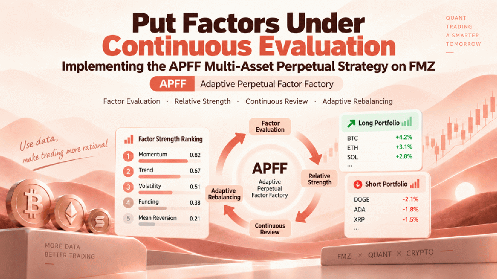
APFF stands for Adaptive Perpetual Factor Factory. It is a multi-asset adaptive factor-factory strategy for perpetual futures. The system compares relative strength across a group of perpetual contracts, combines a small number of interpretable factors into a long-short portfolio, continuously records each factor’s forward performance, gradually adjusts factor weights, and requires new candidates to pass through observation and small-weight trials before they can receive meaningful capital.
This article is based on the repaired and runnable FMZ JavaScript implementation. It walks through the full process from data and factors to actual orders. The corresponding version is v0.1.0, build 20260905-05, research-definition version 2. Current live-running and simulation tests have validated the main engineering workflow, while long-term return performance still requires further out-of-sample evidence.
1. First Turn the Trading Problem Into “Who Is Relatively Stronger?”
At every decision point, APFF works with a cross-section: a group of different contracts observed at the same time.
Suppose two baskets each start with 3,000 USDT of notional exposure. One basket is long and the other is short. Ignoring fees, funding, and rebalancing for the moment, if the long basket rises 4% while the short basket rises 1%, the price PnL is:
Long-basket profit = 3,000 × 4% = 120 USDT
Short-basket loss  = 3,000 × 1% =  30 USDT
Total PnL          = 120 - 30   =  90 USDT
If the long basket falls 2% while the short basket falls 5%, the price PnL can still be positive when both sides have the same notional size. The point is that a long-short portfolio cares about the return spread between two groups of assets.
But similar long and short notionals do not eliminate market risk. If the long side is concentrated in high-volatility assets while the short side is concentrated in low-volatility assets, a sudden market decline can still produce a severe imbalance between the two sides. For that reason, APFF adds volatility scaling, per-symbol caps, and a limited BTC beta hedge on top of relative-strength ranking.
The system operates on several different time scales:
| Task | Current cadence | Purpose |
|---|---|---|
| Best bid/ask, mark price, and other market data | Continuously via WebSocket | Inputs for pricing and data-quality checks |
| Base price factors | Completed 4-hour candles | Avoid using the still-changing current candle |
| Portfolio decisions and research labels | Every 8 hours | Form targets and accumulate the next forward evaluation sample |
| Trading-universe update | Daily | Adapt to changes in market activity |
| Factor evaluation and reweighting | Every 7 days | Reduce the tendency to chase short-term noise |
| Candidate-factor generation | At startup and then every 30 days | Add unregistered candidates from fixed templates |
Market data needs to be timely, but factor weights should move more slowly. Recomputing weights every time the order book ticks would turn a medium/low-frequency portfolio into a noise-chasing rebalancing system.
2. The Trading Universe Determines What the Factors Are Comparing
The current version supports only Binance USDⓈ-M USDT linear perpetual futures, with a default universe size of 30 symbols.
The program reads contract specifications through GetMarkets, while GetTickers and live market data are used to maintain volume, price, and spread information. The base filters include contract trading status, valid quotes, spread limits, and a 90-day listing-age requirement when listing time is available. Eligible contracts are then ranked by current 24-hour trading volume.
A ranking buffer is used to reduce unnecessary membership turnover. By default, an existing member is preferentially retained as long as it remains within the top 40 eligible contracts. The remaining slots are filled with the highest-ranked alternatives. This prevents two contracts with similar volume from repeatedly entering and leaving the portfolio merely because they swap daily ranking positions.
BTC is treated separately as the market benchmark and hedging instrument. Even if it is included in the trading universe, it is excluded from the ordinary alpha ranking. Actual portfolio decisions also require at least 15 non-BTC symbols that pass the data checks. The configured universe size and the number of symbols that are actually usable must therefore be treated as separate quantities.
This implementation has clear boundaries. The current version uses 24-hour trading volume and basic filters. The reference design’s 30-day average volume, historical point-in-time universes, continuous-data completeness filters, and order-book-depth filters have not yet been fully implemented. If listing time is missing, the code also cannot independently prove that a contract has been listed for at least 90 days. These differences should be kept in mind when evaluating strategy results.
3. Five Seed Factors, Each Representing a Testable Hypothesis
The first set of seed factors comes from five families: momentum, reversal, funding, premium, and open interest.
In the table below, RET denotes log price return; RV denotes the sample standard deviation of 4-hour log returns within the corresponding window, not annualized volatility; and Z_TS denotes a time-series z-score computed separately for each symbol.
| Factor | Current calculation | Relationship being tested |
|---|---|---|
| Momentum excluding the latest shock | (RET_7D - RET_4H) / RV_7D | After excluding the latest candle, does medium-term strength persist? |
| Short-term reversal | -RET_4H / RV_24H | Do assets that have fallen excessively in the short term tend to recover? |
| Funding crowding | -Z_TS(funding rate normalized to settlement interval) | Does unusually high funding relative to its own history predict weaker subsequent returns? |
| Premium mean reversion | -Z_TS(Premium series) | Does an unusually high premium relative to its own history tend to mean-revert? |
| OI confirmation | price direction × Z_TS(24H log change in OI notional value) | Does the combination of expanding open-interest notional value and price direction contain predictive information? |
The price-direction term in the OI factor is +1 when the 24-hour return is non-negative and -1 when it is negative. These interpretations are research hypotheses; whether they hold must be answered by mature samples. For example, “high funding” does not mean price must fall immediately. Crowded trades can persist for a long time.
The core of the momentum factor can be seen directly in the source code:
var full = returnBars(prices, p.longBars)
var recent = returnBars(prices, p.skipBars)
var rv = realizedVol(prices, p.longBars)
returnfinite(full) && finite(recent) && rv > 0
    ? direction * (full - recent) / rv
    : NaN
The seed parameters use 42 four-hour candles to represent seven days and skip the most recent candle. Invalid data returns NaN and is then excluded from the valid-value set.
Funding Must First Be Put on a Common Time Scale
Funding settlement intervals can differ across records. The current implementation uses the observed settlement interval to normalize funding rates to a common 8-hour scale before computing time-series z-scores. The seed factor uses roughly 30 days of history and also checks whether historical coverage is sufficient and whether the most recent record is fresh enough.
The current-period funding rate and historical settled funding rates must also be kept separate. FMZ’s GetFundings provides funding-rate data for the current period. APFF stores it as current-period information, while research returns and settlement accounting use separate historical records. See the FMZ GetFundings documentation.
Binance’s /fapi/v1/fundingRate history endpoint provides fundingTime, fundingRate, and the markPrice associated with each funding settlement. This is the basis used by the current implementation to calculate historical funding cash flows. See the Binance USDⓈ-M Futures market-data documentation.
Premium and OI Require Careful Attention to Data Sources
In production, the Premium factor uses historical Premium Index Klines from the exchange. In simulation, the system gradually accumulates a proxy snapshot series based on Mark / Index - 1. The two series are not defined identically, so factor performance observed in the simulated environment cannot be directly treated as evidence for production performance.
Production OI history only accepts the quote-currency notional-value definition. Simulated snapshots are accumulated from available open-interest quantity and price data, then stored in 4-hour time buckets. This avoids accidentally treating six minute-level snapshots as six independent 4-hour observations.
If auxiliary history is insufficient, the corresponding factor can remain unavailable temporarily. For a system designed to run for a long time, explicitly knowing that “this factor does not yet have enough data” is more meaningful than forcing the program to produce a number.
4. Put Every Factor on a Common Ranking Scale So They Can Vote Together
The five raw factors have different units and cannot be added directly. APFF processes each factor cross-sectionally: invalid values are filtered out, the remaining values are winsorized at the 5th and 95th percentiles, and ranks are then mapped to [-1, +1].
If ranks start at 0, the mapping is:
Normalized score = 2 × rank / (number of valid symbols - 1) - 1
The highest score represents the symbol most favored by the factor, while the lowest score represents the least favored one. Equal raw values receive the average rank. If the entire cross-section has no meaningful variation, the factor is treated as invalid so that array ordering cannot manufacture a signal out of nothing.
A single factor must cover at least 80% of the symbols in the current round. When the combined alpha score is formed, each individual symbol must also have coverage from at least 80% of the currently valid factor weight. These two checks separately control whether a factor has enough cross-sectional information and whether a particular symbol has enough combined information.
For a symbol that passes the checks, the combined score is:
Alpha_i = Σ(available factor weight_j × normalized score_ij)
          / Σ(available factor weight_j for symbol i)
This score determines relative ranking. How much capital the portfolio is allowed to use depends on another quantity: the amount of factor budget that is actually available.
5. If Two Factors Are Missing, Why Should Total Exposure Shrink Too?
The five initial seed factors each receive a 20% budget. Suppose momentum, reversal, and funding are available, while Premium and OI have not yet accumulated enough history. The effective factor budget is then:
20% + 20% + 20% = 60%
If the remaining three factors are rescaled to 33.33% each, their weights sum back to 100%, but the same portfolio is now supported by less information and each factor is implicitly carrying more risk.
APFF preserves the original budget meaning of each factor and leaves the unallocated portion idle. The initial gross notional budget is calculated as:
Gross notional budget = account equity
                      × configured gross-exposure ratio
                      × selector confidence factor
                      × sum of effective factor budgets
                      × drawdown scaling factor
Consider an example used only to explain the arithmetic. Account equity is 10,000 USDT, configured gross exposure is 60%, the sum of effective factor budgets is 60%, and both the confidence factor and drawdown factor are 1:
Gross notional budget = 10,000 × 60% × 1 × 60% × 1
                      = 3,600 USDT
Initially, roughly 1,800 USDT is allocated to each side. Per-symbol constraints, hedging constraints, and turnover constraints are applied afterward. This number does not mean that the final orders are guaranteed to fill to the full amount, nor does it represent margin utilization.
Current effective weights are also subject to these caps:
| Budget object | Cap |
|---|---|
| Single ACTIVE factor | 25% |
| Total for one factor family | 35% |
| Single TRIAL factor | 5% |
| All TRIAL factors combined | 10% |
These percentages constrain factor budgets. They further affect portfolio notional exposure and should not be interpreted directly as the percentage of account equity allocated to a particular coin.
The corresponding code is split into two steps. effectiveWeights extracts ACTIVE and TRIAL factors that have valid scores in the current round, then calls the budget-constraint function. The following excerpts show the connection between the two pieces; the second excerpt sits inside the factor loop of normalizeWeightTargets:
functioneffectiveWeights(matrix) {
    var raw = {}
    factorIdsByStatus(["ACTIVE", "TRIAL"]).forEach(function(id) {
        if (Object.keys(matrix[id] || {}).length)
            raw[id] = Math.max(0, num(G.registry[id].weight, 0))
    })
    returnnormalizeWeightTargets(raw, G.registry, true)
}

// Per-factor cap inside normalizeWeightTargetsvar cap = factor.status === "TRIAL"
    ? FIXED.trialFactorCap : FIXED.activeFactorCap
result[id] = Math.min(
    cap,
    Math.max(0, num(raw[id], 0))
        / (preserveBudget ? Math.max(1, total) : total)
)
The key is the final true, which corresponds to preserveBudget. Suppose the sum of valid weights, total, is only 0.6. The denominator becomes Math.max(1, 0.6), so each 0.2 stays 0.2. If the code divided directly by 0.6, each factor would be inflated to approximately 0.3333. If total budget exceeds 1, the same denominator mechanism compresses it back into the total budget range. Later checks also enforce family caps and total trial-factor caps. Any budget clipped by these constraints is not redistributed to the other factors.
6. Save Today’s Decision First, Then Wait for Tomorrow’s Answer
One of the easiest mistakes in an adaptive system is to change the question while evaluating the answer.
Whenever APFF generates a new decision round, it stores the universe version, entry reference prices, factor scores, and coverage observed at that time, then creates a research sample that matures eight hours later. Factor performance is updated only after that sample matures.
After the first startup, seeing “valid samples: 0” in the status panel can be completely normal. Having enough historical candles to calculate momentum and having accumulated complete forward evaluation samples are two different conditions. The five seed factors being marked ACTIVE describes their initial operating status; it does not mean they have already passed a statistical test.
1. Freeze Sample Membership and Maturity Time
At entry, each factor’s research portfolio uses the scores available at that moment to select approximately the top 20% of symbols for the long side and the bottom 20% for the short side. Half of the notional budget is allocated to each side, with equal weights within each side. Tied symbols on a quantile boundary are included together and side-level weights are then redistributed.
At maturity, a symbol cannot simply be removed because its terminal price is missing, followed by reranking and replacement with another symbol. Otherwise, a losing position that happens to have missing data could disappear from the statistics.
The current implementation allows at most a 60-second terminal-price collection window. Once a terminal price has been fixed, it is not replaced by a later price even if funding history arrives late. Funding history may be awaited until five minutes after the original maturity time; if the required data is still incomplete, the entire sample is invalidated.
This puts an explicit bound on timing error, but the label is still a mid-price research approximation. It cannot be treated as the realized return of a passive limit order in a real exchange queue.
2. Price Features and Trading Returns Use Different Return Definitions
Log returns are suitable for momentum and volatility features. For a fixed-quantity linear perpetual position, however, PnL should be calculated using simple price returns plus funding cash flows.
Let the entry reference price be P0, the terminal price be P1, the k-th funding settlement rate be f_k, and its settlement mark price be M_k. The long-side research return per unit of initial notional is:
r_long = P1 / P0 - 1 - Σ(f_k × M_k / P0)
When historical mark prices are available, the code uses this definition. If mark price is unavailable, the funding impact is approximated against the initial notional. Trading fees are not deducted at this stage.
The factor’s long-short research portfolio then aggregates returns using signed weights and subtracts estimated turnover costs:
Turnover   = Σ |new weight_i - old weight_i|
Netreturn = Σ(new weight_i × r_long_i) - Turnover × one-way cost
For example, if a symbol moves from a +5% long weight to a -5% short weight, the absolute weight change is already 10%, which includes both closing the long and opening the short. Multiplying by 2 again would double-count the cost.
7. Make New Factors Pass Through Observation, Trial, and Exit
The current “factor factory” generates candidates from a finite set of templates. The templates cover momentum, reversal, Funding, Premium, OI, price-volume relationships, low-volatility ideas, and multiple lookback horizons.
Each batch can add at most 12 candidates that have not already been registered. Formula type, parameters, and direction together define a fixed identity used for deduplication. Once the template space is exhausted, later batches may generate no new candidates. The current version does not call a large language model online to generate trading code, nor does it perform open-ended formula search.
The main candidate lifecycle is:
| Status | Meaning | Participates in portfolio? |
|---|---|---|
OBSERVING | Accumulating forward research performance | No |
TRIAL | Passed observation requirements and begins an independent trial evaluation | Yes, but with very small weight |
ACTIVE | Fully admitted to the portfolio | Yes, subject to budget constraints |
DORMANT | Trial failed or an active factor has persistently deteriorated | Weight set to zero |
REJECTED | Rejected, for example because it is too similar to an existing factor | No |
The observation stage requires at least 180 valid 8-hour samples, which is about 60 days under ideal continuous conditions. After entering TRIAL, the candidate must independently accumulate at least another 90 valid samples, or roughly 30 days. Missing samples and weekly screening cadence can make the actual calendar time longer.
Trial-stage performance is recorded separately. Good performance accumulated during OBSERVING cannot be carried over to satisfy the TRIAL threshold.
What Does the Evaluation Look At?
The current evaluation mainly examines Rank IC, cost-adjusted long-short returns, subperiod stability, bucket monotonicity, turnover, and data coverage.
Rank IC measures whether the ranking of entry scores agrees with the ranking of subsequent returns. To reduce small-sample optimism, the mean IC is shrunk:
Shrunk mean IC = n / (n + 60) × mean IC
Stability divides the available return series into four time segments and measures how many segments have positive average net returns. This is a four-segment check; it should not be interpreted as having already survived four real calendar quarters or four complete market regimes.
Candidates must not only have positive shrunk IC but also pass a stricter cost test. The base net return has already deducted one estimated cost charge; promotion testing subtracts the same cost once more to check whether the factor remains positive under doubled costs.
The system also uses block bootstrap resampling to examine result stability. Separately, it estimates a tail probability under a zero-mean null and then applies a dependence-adjusted multiple-testing threshold. These two statistics must not be confused. The bootstrap positive-return frequency shown in the status panel describes the resampling results; it is not a “probability of future profitability.”
These rules are intended to reduce the influence of small samples, repeated screening, and accidental winners. Fixed block length, a finite number of resamples, and continuous online screening still introduce approximations and selection bias. The system therefore cannot claim that all false discoveries have been rigorously controlled.
In addition, if the absolute correlation between a candidate’s contemporaneous research returns and those of existing portfolio factors exceeds 0.85, it is treated as highly redundant. At most two candidates from each batch can enter TRIAL, and at most one from the same family can do so. No more than two factors can be in TRIAL simultaneously, and no more than six factors can be ACTIVE.
The basic admission function used during screening is shown below. The original logic is preserved; only line breaks and comments are made clearer:
functionfactorPasses(factor, minimumSamples) {
    var s = summarizeFactor(factor)
    return s.samples >= minimumSamples
        && s.shrunkIc > 0// meanNet already includes the base cost deduction.// Subtract the same cost once more to test doubled costs.
        && s.meanNet - num(s.turnover, 0)
            * G.cfg.oneWayCostBps / 10000 > 0
        && s.stability >= 0.75
        && s.pPositive >= 0.90
        && s.coverage >= 0.98
}
All conditions must be satisfied simultaneously. stability >= 0.75 requires at least three of the four time segments to have positive average net returns. coverage >= 0.98 checks the average factor coverage across evaluation samples, which is stricter than the 80% threshold used for participation in a single round. During the observation stage, the function is called with a 180-sample threshold. During the trial stage, it uses independent trialMetrics and a 90-sample threshold. Even after this function returns true, the caller still checks the relevant multiple-testing criteria, correlation limits, and slot limits. A single true does not mean the factor has automatically been promoted.
8. Adaptive Reweighting Should Respond to Evidence With Restraint
When there are not enough samples, the system uses equal budgets for the seed factors. Only after the adaptive-sample requirements are met are target weights derived from each factor’s evaluation results.
The implementation’s evidence score combines scaled IC, net-return score, stability, and monotonicity, then subtracts turnover and missing-data penalties. It is an internal composite score, not a calibrated probability.
Target weights also take the volatility of factor research returns into account. The old and new target weights are then smoothed:
Smoothed weight = 70% × old weight + 30% × new target weight
During ordinary weekly reweighting, the change in any single factor is limited to 5 percentage points, after which all budget caps are applied again. Factor dormancy and hard constraints can reduce a weight faster, so this smoothing rule should not be interpreted as saying that exposure can only decrease slowly under all circumstances.
Once an ACTIVE factor has accumulated at least 180 valid samples, it enters DORMANT status and its weight is set to zero if both the mean IC and mean net return over the most recent 90 samples are negative. The current logic reduces or disables a factor; it does not automatically reverse the trading direction merely because recent performance has been poor.
Reversing direction is itself a new hypothesis and should be evaluated from scratch. Otherwise, the system can easily end up chasing noise back and forth across the positive and negative sides of a signal that has simply stopped working.
9. From Combined Scores to Executable Target Positions
The live portfolio differs from the equal-weight research baskets used earlier to evaluate individual factors.
The actual portfolio selects assets from both tails of the combined-score ranking. New targets are chosen from roughly the top and bottom 20%, with at most six symbols on each side. Existing targets are preferentially retained as long as they remain within roughly the corresponding 35% region of the ranking, reducing repeated turnover around the selection boundary.
The raw weight within each side is:
raw weight_i ∝ max(0.05, |Alpha_i|) / RV_7D_i
Stronger relative scores receive larger raw weights, while higher historical volatility reduces allocation. A per-symbol cap is then applied, with the default absolute target notional limited to 8% of account equity.
The BTC hedge estimates beta from aligned 4-hour returns. If the absolute estimated beta exposure of the portfolio exceeds 2% of equity, the program attempts to offset it with BTC. The hedge itself is capped and remains subject to per-symbol and total-portfolio exposure limits. Some residual beta can remain after clipping, so this is intentionally a limited hedge.
Turnover is handled last. Under normal target rebalancing, the notional amount changed in one decision is softly capped at 20% of account equity. If the desired adjustment exceeds that level, the portfolio moves proportionally toward the new target. However, if the current target already violates a hard risk limit, required deleveraging takes priority; excessive risk is not preserved merely to satisfy the turnover limit.
After all hedge and turnover adjustments, the program performs another check of per-symbol and total exposure. A target that passed earlier checks can become invalid again after subsequent transformations, so this final validation must occur before the executable target is finalized.
Because the actual portfolio uses volatility weighting, ranking buffers, BTC hedging, and turnover controls, individual factor research returns cannot simply be added together and treated as strategy-level account returns. The research layer evaluates ranking information; the execution layer must additionally determine whether that information can be converted into positions at a reasonable cost.
10. After an Order Fills, the Position Still Has to Give the Same Answer
Once a multi-asset strategy runs asynchronously, market data, order responses, fills, and position snapshots can arrive in different orders.
FMZ’s exchange.Go can call trading interfaces asynchronously and retrieve results through the returned object’s wait method. APFF uses this mechanism to stagger data and account queries. The current maximum number of concurrent tasks is 8. See the FMZ exchange.Go documentation.
Asynchronous execution creates another question that must be answered explicitly: did this request actually take effect on the exchange?
Save the Intent Before Sending the Order
Before every order is sent, the program first generates a client order ID and records the symbol, side, quantity, current position, and corresponding target, then persists that intent. If persistence fails, the order is not sent.
At most one active intent is allowed per symbol, and at most four can exist globally at the same time. When reversing direction, the program closes the original side before considering a new position on the opposite side. Normal execution uses GTX passive limit orders. New targets have a default execution window of 15 minutes. After that window expires, the strategy stops adding new risk, while required risk reduction and reconciliation continue.
If a Request Times Out, Verify the Result First
A definite rejection and an unknown result must be treated differently. Insufficient balance, precision errors, and similar responses can be handled as explicit rejections. A timeout, broken connection, or unknown response may occur after the exchange has already accepted the order.
The current implementation continuously reconciles by order ID or client order ID against order details, open orders, and historical orders. It does not release an unknown intent and submit the order again merely because “the open-order list is empty” or “tens of seconds have passed.”
After the Order Reaches a Terminal State, Confirm the Position Too
Suppose the original position is 100 contracts and a closing sell order accumulates 30 contracts of fills. The next position snapshot should confirm that roughly 70 contracts remain. This query must be initiated after the order reaches its terminal state; a late response from an older request cannot be used as confirmation. If the snapshot still reports 100 contracts, the program shows WAIT_POSITION, continues querying, and keeps the symbol locked.
The expected position is calculated as “initial position + signed cumulative filled quantity” and stored as barrier.expected. After a position response arrives, applyPositions checks whether the reconciliation lock can be released. The following excerpt shows the core order path in the current version, omitting diagnostic logs and legacy state-migration branches. positions is the already-parsed position map:
var snapshotAt = num(requestedAt, nowMs())
Object.keys(G.execution.positionBarriers || {}).forEach(function(symbol) {
    var barrier = G.execution.positionBarriers[symbol]
    // The query must have been initiated after the terminal state.// A symbol with simultaneous long and short positions cannot be unlocked.if (snapshotAt <= barrier.at || (G.actual.hedgedSymbols || {})[symbol])
        returnvar spec = G.universe.markets[symbol]
    var tolerance = Math.max(1e-12, num(spec && spec.step, 0) / 2)
    if (finite(barrier.expected)
        && Math.abs(num(positions[symbol], 0) - barrier.expected) > tolerance)
        returndelete G.execution.positionBarriers[symbol]
    clearIssue("POSITION_RECONCILE_" + symbol)
})
snapshotAt uses the request-initiation time to determine ordering. Quantity comparison allows an error of half the order-size step and also applies a tiny numerical-error floor. If any check fails, the function returns early, the symbol lock remains in place, and the execution layer continues blocking new orders for that symbol. Only after all checks pass is positionBarriers[symbol] deleted. This avoids the classic duplicate-trading failure mode of “the order has filled, the position endpoint has not updated yet, so the strategy sends the same trade again.”
One Binance simulation test provides a concrete example. A TAC position-reduction order accumulated 17,990 contracts of fills, reducing the position from 37,062 to 19,072 contracts. During the process, a cancel request raced with the fill and produced one -2011 response. Subsequent order queries confirmed the remaining execution within about 2.17 seconds, completing reconciliation.
This test record shows how that particular race condition was recovered. The error message itself cannot prove that the order filled, nor can it prove that cancellation succeeded. Final confirmation still requires the terminal order state and the position quantity to agree with each other.
11. Risk Controls Must Work While the Program Is Still Running
APFF scales target budget according to drawdown from the historical equity peak:
| Equity drawdown | Target-budget scaling |
|---|---|
| Less than 4% | 100% |
| At least 4%, less than 7% | 70% |
| At least 7%, less than 10% | 40% |
| At least 10% | Target set to zero; new risk is paused |
The 4% and 7% tiers take effect on the current target immediately; the system does not wait for the next 8-hour decision. The zero-target state continues to prevent new exposure, while the execution layer reduces positions after it obtains the required market and account state. These controls constrain the program’s targets and execution behavior; they do not guarantee that maximum loss in an extreme market will stop exactly at 10%.
The interactive controls distinguish three actions: PAUSE_NEW pauses new risk, RESUME resumes portfolio execution, and REDUCE_TO_ZERO cancels this strategy’s orders, completes reconciliation, and then closes the positions managed by this strategy.
The strategy uses its own position-ownership markers to determine what it manages. If a target symbol already has a position that is not attributed to this strategy, or if simultaneous long and short positions are detected in the same symbol, automatic trading for that symbol is blocked.
Stopping the process does not automatically liquidate positions. If the intention is to flatten the portfolio, the flattening workflow should be allowed to complete and its result should be verified. Simply stopping the robot leaves positions in place. For a multi-asset portfolio, this distinction directly determines how much risk remains in the account after shutdown.
12. How to Interpret Run Modes and the Status Panel on FMZ
The current version provides three run modes:
| Mode | Behavior | Meaning of the displayed return |
|---|---|---|
SHADOW | Reads public market data and computes factors, research performance, and portfolio targets | No simulated fills; no trading-account return |
PAPER | Simulates fills locally using live Bid/Ask, and records positions, fees, and funding | Return from the local simulated ledger |
LIVE | Reads the configured exchange account and sends orders | Change in equity of the connected account |
LIVE uses the trading interface. If the exchange object is configured for the Binance simulated environment, orders are matched in the exchange’s simulation environment. Only when the strategy is connected to a real-money account does LIVE correspond to real-money trading. Both the run-mode name and the account environment must be checked.
The current program depends on live WebSocket data and blocks entry into FMZ’s historical backtest environment during initialization. Therefore, PAPER must accumulate forward results through real-time running. It is not a mode where one can simply select a historical date range and backtest it.
After importing the complete strategy file and adding a corresponding Binance futures exchange object, the main parameters are:
| Parameter | Default | Meaning |
|---|---|---|
RunMode | PAPER | Run mode |
UniverseSize | 30 | Target number of symbols in the trading universe |
GrossExposurePct | 60 | Configured budget for the sum of absolute long and short notional relative to equity |
MaxSymbolPct | 8 | Maximum absolute target notional for a single symbol as a percentage of equity |
EstimatedOneWayCostBps | 4 | Estimated one-way cost; 4 bps = 0.04% |
LiveConfirm | empty | LIVE requires the exact text ENABLE_APFF_LIVE |
These values are program defaults and have not been certified as return-optimal parameters. Cost parameters in particular must be interpreted according to the run mode. The research layer deducts estimated cost from reference-price returns. In PAPER, buys use the Ask and sells use the Bid, so bid-ask spread is already reflected; the configured cost parameter is then charged additionally as a fee estimate. Cost calibration should avoid counting the same cost component twice.
When observing the strategy, the status panel can be read in this order:
- Market data and data gates: Are both market-data connections updating continuously, and are enough tradable symbols available?
- Research samples and maturity: Is the system merely warmed up on data, or has it already accumulated valid forward samples?
- Configured weights and effective target weights: Which factors are actually participating in this round?
- Targets and positions: Are deviations caused by the execution window, minimum order notional, exchange limits, or fills that are still awaiting confirmation?
- Order intents and position-confirmation locks: Are
UNKNOWNorWAIT_POSITIONstates persisting, and are the related reconciliation queries still progressing?
The PAPER ledger separates realized PnL, unrealized PnL, funding, and estimated fees. Funding is posted against the historical position that existed at settlement time; late-arriving funding records are not simply applied to the current position.
LIVE currently displays performance mainly as the difference between account equity and baseline account equity. It does not yet fully exclude deposits, withdrawals, or the effect of other strategies, and it does not fully separate actual realized PnL, unrealized PnL, and funding. Items that are not separately accounted for are shown as -; they must not be interpreted as zero.
13. What Has Been Validated So Far?
As of the build used in this article, the project has completed base logic checks, 23 order-regression checks, and 34 dedicated audit tests. The dedicated tests include 36 accelerated decision cycles and 500 randomized weight-constraint checks.
It is important to state what these numbers do and do not mean. The 36 cycles use synthetic data and a controlled clock to validate sampling, maturity, accounting, and recovery workflows; they are not a 12-day historical return backtest. The randomized constraint checks validate budget caps; they do not validate the predictive power of the factors.
Runtime retesting in the Binance simulated environment covers actual simulated matching, restart recovery, cancel/fill races, explicit order rejection, and position reconciliation. These results are enough to justify continuing to accumulate forward evidence, but they are not sufficient to report conclusions about annualized return, Sharpe ratio, or long-term win rate.
The highest-priority next steps are to add point-in-time historical data and independent rolling out-of-sample validation, calibrate execution costs by symbol and market regime, add correlation-cluster position limits, and introduce an entry threshold requiring expected return to cover trading costs. These directions already exist in the research design, but they have not all been fully implemented in the current code.
APFF has already encoded the lifecycle of a factor—from creation and performance recording, to receiving budget, participating in orders, and eventually leaving the portfolio—into a running program. The most valuable data from here will be the decision recorded at each point in time and the answer obtained eight hours later under the same rules: which signals remain effective, which work only in certain market regimes, and how much of their apparent edge survives actual execution.