A Powerful Tool for Programmatic Traders: Incremental Update Algorithm for Calculating Mean and Variance

Introduction

In programmatic trading, it is often necessary to calculate averages and variances, such as calculating moving averages and volatility indicators. When we need high-frequency and long-term calculations, it's necessary to retain historical data for a long time, which is both unnecessary and resource-consuming. This article introduces an online updating algorithm for calculating weighted averages and variances, which is particularly important for processing real-time data streams and dynamically adjusting trading strategies, especially high-frequency strategies. The article also provides corresponding Python code implementation to help traders quickly deploy and apply the algorithm in actual trading.

Simple Average and Variance

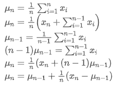
If we use

to represent the average value of the nth data point, assuming that we have already calculated the average of n-1 data points

, now we receive a new data point

. We want to calculate the new average number

including the new data point. The following is a detailed derivation.

The variance update process can be broken down into the following steps:

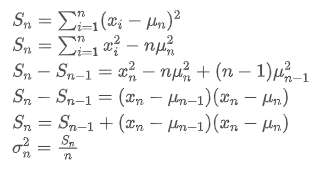
As can be seen from the above two formulas, this process allows us to update new averages and variances upon receiving each new data point

by only retaining the average and variance of the previous data, without saving historical data, making calculations more efficient. However, the problem is that what we calculate in this way are the mean and variance of all samples, while in actual strategies, we need to consider a certain fixed period. Observing the above average update shows that the amount of new average updates is a deviation between new data and past averages multiplied by a ratio. If this ratio is fixed, it will lead to an exponentially weighted average, which we will discuss next.

Exponentially-weighted mean

The exponential weighted average can be defined by the following recursive relationship:

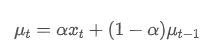
Among them,

is the exponential weighted average at time point t,

is the observed value at time point t, α is the weight factor, and

is the exponential weighted average of the previous time point.

Exponentially-weighted variance

Regarding variance, we need to calculate the exponential weighted average of squared deviations at each time point. This can be achieved through the following recursive relationship:

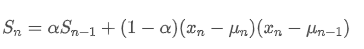
Among them,

is the exponential weighted variance at time point t, and

is the exponential weighted variance of the previous time point.

Observe the exponentially weighted average and variance, their incremental updates are intuitive, retaining a portion of past values and adding new changes. The specific derivation process can be referred to in this paper: stats.pdf

SMA and EMA

The SMA (also known as the arithmetic mean) and EMA are two common statistical measures, each with different characteristics and uses. The former one assigns equal weight to each observation, reflecting the central position of the data set. The latter one is a recursive calculation method that gives higher weight to more recent observations. The weights decrease exponentially as the distance from current time increases for each observation.

Weight distribution: The SMA assigns the same weight to each data point, while the EMA gives higher weight to the most recent data points.
Sensitivity to new information: The SMA is not sensitive enough to newly added data, as it involves recalculating all data points. The EMA, on the other hand, can reflect changes in the latest data more quickly.
Computational complexity: The calculation of the SMA is relatively straightforward, but as the number of data points increases, so does the computational cost. The computation of the EMA is more complex, but due to its recursive nature, it can handle continuous data streams more efficiently.

Approximate Conversion Method Between EMA and SMA

Although SMA and EMA are conceptually different, we can make the EMA approximate to a SMA containing a specific number of observations by choosing an appropriate α value. This approximate relationship can be described by the effective sample size, which is a function of the weight factor α in the EMA.

SMA is the arithmetic average of all prices within a given time window. For a time window N, the centroid of the SMA (i.e., the position where the average number is located) can be considered as:

the centroid of SMA

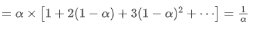
EMA is a type of weighted average where the most recent data points have greater weight. The weight of EMA decreases exponentially over time. The centroid of EMA can be obtained by summing up the following series:

the centroid of EMA

When we assume that SMA and EMA have the same centroid, we can obtain:

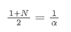
To solve this equation, we can obtain the relationship between α and N.

This means that for a given SMA of N days, the corresponding α value can be used to calculate an "equivalent" EMA, so that they have the same centroid and the results are very similar.

Conversion of EMA with Different Update Frequencies

Assume we have an EMA that updates every second, with a weight factor of

. This means that every second, the new data point will be added to the EMA with a weight of

, while the influence of old data points will be multiplied by

If we change the update frequency, such as updating once every f seconds, we want to find a new weight factor

, so that the overall impact of data points within f seconds is the same as when updated every second.

Within f seconds, if no updates are made, the impact of old data points will continuously decay f times, each time multiplied by

. Therefore, the total decay factor after f seconds is

In order to make the EMA updated every f seconds have the same decay effect as the EMA updated every second within one update period, we set the total decay factor after f seconds equal to the decay factor within one update period:

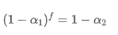
Solving this equation, we obtain new weight factors

This formula provides the approximate value of the new weight factor , which maintains the EMA smoothing effect unchanged when the update frequency changes. For example: When we calculate the average price with a value of 0.001 and update it every 10 seconds, if it is changed to an update every second, the equivalent value would be approximately 0.01.

Implementation of Python Code

classExponentialWeightedStats:
    def__init__(self, alpha):
        self.alpha = alpha
        self.mu = 0
        self.S = 0
        self.initialized = Falsedefupdate(self, x):
        ifnot self.initialized:
            self.mu = x
            self.S = 0
            self.initialized = Trueelse:
            temp = x - self.mu
            new_mu = self.mu + self.alpha * temp
            self.S = self.alpha * self.S + (1 - self.alpha) * temp * (x - self.mu)
            self.mu = new_mu

    @propertydefmean(self):
        return self.mu

    @propertydefvariance(self):
        return self.S

# Usage example
alpha = 0.05# Weight factor
stats = ExponentialWeightedStats(alpha)
data_stream = [] # Data streamfor data_point in data_stream:
    stats.update(data_point)

Summary

In high-frequency programmatic trading, the rapid processing of real-time data is crucial. To improve computational efficiency and reduce resource consumption, this article introduces an online update algorithm for continuously calculating the weighted average and variance of a data stream. Real-time incremental updates can also be used for various statistical data and indicator calculations, such as the correlation between two asset prices, linear fitting, etc., with great potential. Incremental updating treats data as a signal system, which is an evolution in thinking compared to fixed-period calculations. If your strategy still includes parts that calculate using historical data, consider transforming it according to this approach: only record estimates of system status and update the system status when new data arrives; repeat this cycle going forward.