The Beginning of It All
I’ve been involved in quantitative trading for a while now. To be honest, most of the time I just experiment with strategies shared by others—tweaking parameters here and there to see what happens. Rarely do I get the chance to build a strategy entirely from scratch. It’s mostly because I don’t often have a solid idea to start with, and even when I do, the gap between a concept and actual code always feels pretty wide.
A while ago, while I had some free time, I found myself browsing Bilibili again. I stumbled across a livestream by “watsonzhang” covering stock trading. I was watching casually at first, but unexpectedly, something he said sparked an idea.
That One Brilliant Comment
While watsonzhang was explaining the KDJ indicator, a comment in the chat caught my attention. Someone wrote:
“If the hook after a small drop forms quickly, the price might go up later. If the hook after a big drop forms slowly, there’s likely more downside. If a hook forms quickly after a small rise, a drop may follow. If it forms slowly after a strong rise, the uptrend might continue.”
I paused for a moment—what an insightful summary! Just one sentence, but it captured the behavior of the J value in the KDJ indicator with remarkable clarity.
Now, watsonzhang focuses on stocks, but I couldn’t help thinking: could this logic apply to crypto markets as well? The more I thought about it, the more it made sense. Combining the magnitude of price movements with the speed of indicator response seems like a reasonable way to assess potential future trends. And since crypto markets trade 24/7 and tend to be more volatile, this framework might even perform better there.
At that moment, I got excited. It felt like I had finally found a direction worth exploring. But right after that came the familiar problem: how do I turn this idea into code? In the past, I probably would’ve let it go or shelved it for “later” — which usually meant never.
Taking the First Step
But this time felt different. I remembered the AI assistant on the FMZ platform and thought, why not see if it can help “translate” this concept into actual code?
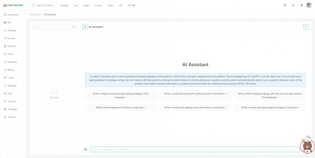
With a “let’s just see what happens” mindset, I opened up the AI assistant on the FMZ platform and typed in the idea exactly as it came to me. I also added a note saying that the original theory was based on stocks, but I wanted to try applying it to cryptocurrencies instead.
To my surprise, the AI understood it almost instantly and quickly generated a complete set of strategy code. I was honestly a bit shocked — like, has AI really come this far?
First Version of the Strategy Code:
/*backtest
start: 2024-07-18 09:40:00
end: 2025-06-30 15:00:00
period: 1h
basePeriod: 1h
exchanges: [{"eid":"Binance","currency":"BTC_USDT"}]
*///@version=5strategy("KDJ J value change speed strategy", overlay=false)

// Input parameters - optimized for the cryptocurrency market
kdj_length = input.int(14, "KDJ period", minval=1)
k_smooth = input.int(3, "K smooth", minval=1)
d_smooth = input.int(3, "D smooth", minval=1)
j_speed_period = input.int(5, "J value change speed calculation period", minval=1)
price_change_threshold = input.float(3.0, "Price change threshold (%) - Distinguish between large and small changes", minval=0.1) / 100
j_speed_threshold = input.float(12.0, "J value change speed threshold - distinguish fast and slow", minval=0.1)
j_change_threshold = input.float(1.5, "J value changes ignore threshold - filter noise", minval=0.1)
price_change_ignore_threshold = input.float(0.5, "Price change ignore threshold (%) - filter noise", minval=0.01) / 100// Cryptocurrency risk control parameters
max_consecutive_trades = input.int(5, "Maximum number of consecutive transactions", minval=1)
min_bars_between_signals = input.int(3, "Minimum interval between signals", minval=1)
enable_stop_loss = input.bool(true, "Enable stop loss")
stop_loss_pct = input.float(5.0, "Stop loss percentage (%)", minval=0.5) / 100// Calculating the KDJ indicator
highest_high = ta.highest(high, kdj_length)
lowest_low = ta.lowest(low, kdj_length)
rsv = (close - lowest_low) / (highest_high - lowest_low) * 100

k = ta.sma(rsv, k_smooth)
d = ta.sma(k, d_smooth)
j = 3 * k - 2 * d

// Calculate the continuous change speed of J value// Count the cumulative change and duration of continuous rise or fallvarfloat j_cumulative_change = 0.0varint j_consecutive_bars = 0varint j_direction = 0// 1 is rising, -1 is falling, 0 is the initial

j_current_change = j - j[1]
// Only when the change exceeds the threshold is it considered directional
j_current_direction = math.abs(j_current_change) > j_change_threshold ?
                     (j_current_change > 0 ? 1 : -1) : 0// Check if the J value direction changesif j_current_direction != j_direction and j_current_direction != 0// Change direction, restart statistics
    j_cumulative_change := math.abs(j_current_change)
    j_consecutive_bars := 1
    j_direction := j_current_direction
elseif j_current_direction == j_direction and j_current_direction != 0// Same direction, cumulative change
    j_cumulative_change += math.abs(j_current_change)
    j_consecutive_bars += 1elseif j_current_direction == 0// Changes are too small to be ignored, but time continues to accumulate
    j_consecutive_bars += 1// J value change speed = cumulative change / duration
j_speed = j_consecutive_bars > 0 ? j_cumulative_change / j_consecutive_bars : 0// Calculate the continuous price change range// Count the cumulative change and duration of continuous rise or fallvarfloat price_cumulative_change = 0.0varint price_consecutive_bars = 0varint price_direction = 0// 1 is rising, -1 is falling, 0 is the initial

price_current_change = (close - close[1]) / close[1]
// Only when the change exceeds the threshold, is it considered directional
price_current_direction = math.abs(price_current_change) > price_change_ignore_threshold ?
                         (price_current_change > 0 ? 1 : -1) : 0// Detect if the price direction has changedif price_current_direction != price_direction and price_current_direction != 0// Change direction, restart statistics
    price_cumulative_change := math.abs(price_current_change)
    price_consecutive_bars := 1
    price_direction := price_current_direction
elseif price_current_direction == price_direction and price_current_direction != 0// Same direction, cumulative change
    price_cumulative_change += math.abs(price_current_change)
    price_consecutive_bars += 1elseif price_current_direction == 0// Changes are too small to be ignored, but time continues to accumulate
    price_consecutive_bars += 1// Price change = Cumulative change
price_change = price_cumulative_change

// Determine the type of price change
is_small_change = price_change < price_change_threshold
is_large_change = price_change >= price_change_threshold

// Determine the price direction (based on the current continuous change direction)
is_price_up = price_direction == 1
is_price_down = price_direction == -1// Determine the speed of change of J value
is_j_fast = j_speed > j_speed_threshold
is_j_slow = j_speed <= j_speed_threshold

// Transaction control variablesvarfloat entry_price = 0.0// Strategy signal logic// 1. A small drop will cause the hook to drop quickly, which may lead to a bullish trend in the future
signal_small_down_fast_j = is_small_change and is_price_down and is_j_fast

// 2. If the price drops sharply, it will drop slowly, and it will fall further in the later period.
signal_large_down_slow_j = is_large_change and is_price_down and is_j_slow

// 3. The small upward trend grows fast, which may lead to a bearish trend in the later period
signal_small_up_fast_j = is_small_change and is_price_up and is_j_fast

// 4. The sharp rise is slow, and there may be further rises in the later period
signal_large_up_slow_j = is_large_change and is_price_up and is_j_slow

// Trading signals
long_signal = (signal_small_down_fast_j or signal_large_up_slow_j)
short_signal = (signal_small_up_fast_j or signal_large_down_slow_j)

// Execute transactionsif long_signal andstrategy.position_size == 0strategy.entry("Long", strategy.long, comment="Long signal to open a position")
    entry_price := closeif short_signal andstrategy.position_size == 0strategy.entry("Short", strategy.short, comment="Short signal to open a position")
    entry_price := close// Closing conditions// 1. Close the position upon signal reversalifstrategy.position_size > 0and short_signal
    strategy.close("Long", comment="Signal reversal to close long position")


ifstrategy.position_size < 0and long_signal
    strategy.close("Short", comment="Signal reversal to close short position")


// 2. Stop loss and close positionif enable_stop_loss
    ifstrategy.position_size > 0andclose <= entry_price * (1 - stop_loss_pct)
        strategy.close("Long", comment="Stop loss to close long positions")


    ifstrategy.position_size < 0andclose >= entry_price * (1 + stop_loss_pct)
        strategy.close("Short", comment="Stop loss to close short positions")


// Plot indicatorsplot(j, "J value", color=color.blue, linewidth=2)
hline(80, "Overbought line", color=color.red, linestyle=hline.style_dashed)
hline(20, "Oversold line", color=color.green, linestyle=hline.style_dashed)
hline(50, "Midline", color=color.gray, linestyle=hline.style_dotted)

// Plot signal markersplotshape(signal_small_down_fast_j, title="Small drop and quick hook - bullish", location=location.belowbar, color=color.lime, style=shape.triangleup, size=size.small,overlay=true)
plotshape(signal_large_down_slow_j, title="Large drop slow hook-bearish", location=location.belowbar, color=color.red, style=shape.triangledown, size=size.small,overlay=true)
plotshape(signal_small_up_fast_j, title="Small up and fast hook - bearish", location=location.abovebar, color=color.red, style=shape.triangledown, size=size.small,overlay=true)
plotshape(signal_large_up_slow_j, title="Large rise slow hook-bullish", location=location.abovebar, color=color.lime, style=shape.triangleup, size=size.small,overlay=true)
The First Wave of Excitement and Disappointment
The first thing I did after getting the code was check whether it would actually run. The FMZ platform’s editor showed no syntax errors, which was a relief.
Then came the most exciting part — on line backtesting. On the AI assistant page, there’s an option in the bottom-right corner of the generated page to run live backtests. I selected BTC as the trading pair, set the time range, and hit the backtest button with anticipation.
When the results came out, my feelings were mixed. The code did run successfully, and the logic seemed sound—but the backtest results were underwhelming. While there were some profitable trades, the overall win rate was low, and there were frequent streaks of losses.
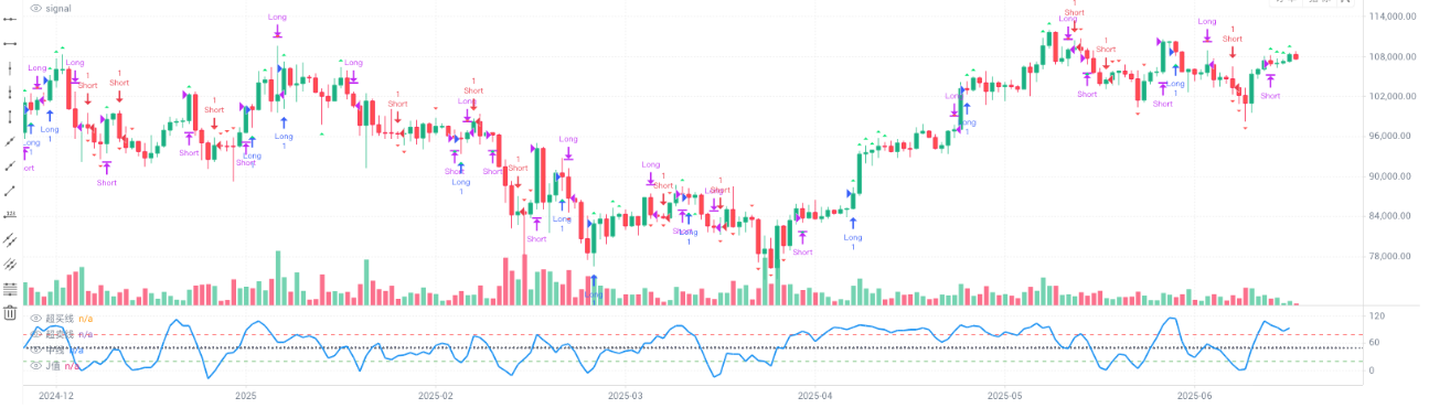
It felt like building a plane that should fly in theory—only to watch it stay grounded in reality. A bit disappointing, but I wasn’t ready to give up just yet.
Deep in Thought
If the theory made sense and the code could run, then where was the problem?
I started digging into the logic of the code more carefully. I noticed that the AI’s implementation mainly focused on calculating the rate of change of the J value to determine whether the “hook” was forming quickly or slowly:
j_speed = j_cumulative_change / j_consecutive_bars
is_j_fast = j_speed > j_speed_threshold
is_j_slow = j_speed <= j_speed_threshold
At first glance, everything looked fine—but something felt off.
After thinking it over for a while, I suddenly realized the issue: the calculation was only looking at the rate of change at a single moment in time. It didn’t take into account the continuity of the change.
For example, the J value might spike sharply on one day, but if that change is short-lived and it returns to normal the next day, relying on that single data point could be misleading.
The original theory talked about “hooking quickly” or “hooking slowly” — and that “quick” or “slow” was describing an ongoing process, not just a snapshot in time.
Looking for a Breakthrough
Once I realized that, I got excited again. It felt like I had identified the missing piece — but I still wasn’t sure how to adjust the code to reflect it.
Then I remembered seeing some comments before where people mentioned the importance of tracking indicator changes over time. That’s it — continuity! That was exactly what I had just been thinking about.
So I went back to the AI assistant—this time with a more specific request: I wanted it to focus on the continuity of changes in the J value. Instead of just looking at the rate of change on a single day, the goal was to evaluate the trend over several consecutive days.
The solution the AI provided genuinely impressed me. It completely redesigned the logic behind analyzing the J value:
- It not only recorded the current direction of change but also tracked how many consecutive days the change persisted.
- A trend was only considered valid if the J value moved consistently in the same direction for several days.
- Once continuity was confirmed, it would then assess whether the rate of change was “fast” or “slow” based on that sustained trend.
Second Version – Improved Strategy Code:
/*backtest
start: 2024-07-18 09:40:00
end: 2025-06-30 15:00:00
period: 1h
basePeriod: 1h
exchanges: [{"eid":"Binance","currency":"BTC_USDT"}]
*///@version=5strategy("KDJ J value continuous change strategy", overlay=false)
//Input parameters
kdj_length = input.int(9, "KDJ period", minval=1)
k_smooth = input.int(3, "K smooth", minval=1)
d_smooth = input.int(3, "D smooth", minval=1)
j_speed_period = input.int(3, "J value change speed calculation period", minval=1)
price_change_threshold = input.float(1.5, "Price change threshold (%) - Distinguish between large and small changes", minval=0.1) / 100
j_fast_threshold = input.float(15.0, "J value rapid change threshold", minval=1.0)
j_slow_threshold = input.float(5.0, "J value slow change threshold", minval=0.1)
j_change_threshold = input.float(1.0, "J value changes ignore threshold - filter noise", minval=0.1)
price_change_ignore_threshold = input.float(0.2, "Price change ignore threshold (%) - filter noise", minval=0.01) / 100
min_consecutive_bars = input.int(3, "Minimum number of consecutive K lines", minval=2)
// Risk control parameters
max_consecutive_trades = input.int(3, "Maximum number of consecutive transactions", minval=1)
min_bars_between_signals = input.int(5, "Minimum interval between signals", minval=1)
enable_stop_loss = input.bool(true, "Enable stop loss")
stop_loss_pct = input.float(3.0, "Stop loss percentage (%)", minval=0.5) / 100// Calculating the KDJ indicator
highest_high = ta.highest(high, kdj_length)
lowest_low = ta.lowest(low, kdj_length)
rsv = (close - lowest_low) / (highest_high - lowest_low) * 100
k = ta.sma(rsv, k_smooth)
d = ta.sma(k, d_smooth)
j = 3 * k - 2 * d
// Improved analysis of J value continuity changevarfloat j_cumulative_change = 0.0// Cumulative change that maintains direction (positive or negative)varint j_consecutive_bars = 0varint j_direction = 0// 1 means continuous rise, -1 means continuous fall, 0 means no clear directionvarfloat j_start_value = 0.0
j_current_change = j - j[1]
// Only when the change exceeds the threshold is it considered directional
j_current_direction = math.abs(j_current_change) > j_change_threshold ?
(j_current_change > 0 ? 1 : -1) : 0// Redesigned J value continuity detection logicif j_current_direction != 0if j_current_direction == j_direction
// The direction is the same, continue to accumulate (keep the positive and negative signs)
j_cumulative_change += j_current_change
j_consecutive_bars += 1else// Change direction, restart statistics
j_cumulative_change := j_current_change
j_consecutive_bars := 1
j_direction := j_current_direction
j_start_value := j[1]
else// If the change is minimal, it's considered sideways movement, and the continuity counter is reset.if j_consecutive_bars > 0
j_consecutive_bars += 1else
j_cumulative_change := 0.0
j_consecutive_bars := 0
j_direction := 0// Calculate the J-value continuity indicator (maintain directionality)
j_total_change = j - j_start_value // Total change from the starting point to the current point (signed)
j_avg_speed = j_consecutive_bars > 0 ? j_cumulative_change / j_consecutive_bars : 0// Average rate of change (signed)
j_abs_avg_speed = math.abs(j_avg_speed) // The absolute value of the change rate// New J value change judgment logic
is_j_continuous_up = j_direction == 1and j_consecutive_bars >= min_consecutive_bars
is_j_continuous_down = j_direction == -1and j_consecutive_bars >= min_consecutive_bars
// Speed judgment based on continuity and change amplitude
is_j_fast_up = is_j_continuous_up and j_abs_avg_speed > j_fast_threshold
is_j_slow_up = is_j_continuous_up and j_abs_avg_speed <= j_slow_threshold and j_abs_avg_speed > 0
is_j_fast_down = is_j_continuous_down and j_abs_avg_speed > j_fast_threshold
is_j_slow_down = is_j_continuous_down and j_abs_avg_speed <= j_slow_threshold and j_abs_avg_speed > 0// Calculate the continuous price change range (keep the original logic)varfloat price_cumulative_change = 0.0varint price_consecutive_bars = 0varint price_direction = 0
price_current_change = (close - close[1]) / close[1]
price_current_direction = math.abs(price_current_change) > price_change_ignore_threshold ?
(price_current_change > 0 ? 1 : -1) : 0if price_current_direction != price_direction and price_current_direction != 0
price_cumulative_change := math.abs(price_current_change)
price_consecutive_bars := 1
price_direction := price_current_direction
elseif price_current_direction == price_direction and price_current_direction != 0
price_cumulative_change += math.abs(price_current_change)
price_consecutive_bars += 1elseif price_current_direction == 0
price_consecutive_bars += 1
price_change = price_cumulative_change
// Determine the type of price change
is_small_change = price_change < price_change_threshold
is_large_change = price_change >= price_change_threshold
is_price_up = price_direction == 1
is_price_down = price_direction == -1// Transaction control variablesvarfloat entry_price = 0.0// Redesigned the strategy signal logic to emphasize the continuity of J value// 1. A small drop + J value continues to quickly hook down = bullish (the downward inertia weakens, and the J value falls back quickly)
signal_small_down_fast_j_down = is_small_change and is_price_down and is_j_fast_down
// 2. Sharp decline + J value continues to slowly hook down = bearish (the downward momentum is still there, and the J value is declining slowly)
signal_large_down_slow_j_down = is_large_change and is_price_down and is_j_slow_down
// 3. Slight increase + J value continues to rise quickly = bearish (the upward inertia weakens, and the J value falls quickly)
signal_small_up_fast_j_up = is_small_change and is_price_up and is_j_fast_up
// 4. A sharp rise + J value continues to rise slowly = bullish (the upward momentum is still there, and the J value continues to rise)
signal_large_up_slow_j_up = is_large_change and is_price_up and is_j_slow_up
// Trading signals
long_signal = (signal_small_down_fast_j_down or signal_large_up_slow_j_up)
short_signal = (signal_small_up_fast_j_up or signal_large_down_slow_j_down)
// Execute transactionsif long_signal andstrategy.position_size == 0strategy.entry("Long", strategy.long, comment="Long signal to open a position")
entry_price := closeif short_signal andstrategy.position_size == 0strategy.entry("Short", strategy.short, comment="Short signal to open a position")
entry_price := close// Closing conditionsifstrategy.position_size > 0and short_signal
strategy.close("Long", comment="Signal reversal to close long position")
ifstrategy.position_size < 0and long_signal
strategy.close("Short", comment="Signal reversal to close short position")
// Stop loss closingif enable_stop_loss
ifstrategy.position_size > 0andclose <= entry_price * (1 - stop_loss_pct)
strategy.close("Long", comment="Stop loss to close long positions")
ifstrategy.position_size < 0andclose >= entry_price * (1 + stop_loss_pct)
strategy.close("Short", comment="Stop loss to close short positions")
// Plot indicatorsplot(j, "J value", color=color.blue, linewidth=2)
hline(80, "Overbought Line", color=color.red, linestyle=hline.style_dashed)
hline(20, "Oversold Line", color=color.green, linestyle=hline.style_dashed)
hline(50, "Midline", color=color.gray, linestyle=hline.style_dotted)
// The continuity indicator is shown in the lower sub-chartplot(j_consecutive_bars, "Number of consecutive K lines", color=color.orange)
plot(j_avg_speed, "Average speed of change (with direction)", color=color.purple)
plot(j_abs_avg_speed, "Average change rate (absolute value)", color=color.yellow)
// Plot signal markersplotshape(signal_small_down_fast_j_down, title="Small drop + J quick hook - bullish", location=location.belowbar, color=color.lime, style=shape.triangleup, size=size.small, overlay=true)
plotshape(signal_large_down_slow_j_down, title="Large drop + J slow hook - bearish", location=location.belowbar, color=color.red, style=shape.triangledown, size=size.small, overlay=true)
plotshape(signal_small_up_fast_j_up, title="Small rise + J quick hook - bearish", location=location.abovebar, color=color.red, style=shape.triangledown, size=size.small, overlay=true)
plotshape(signal_large_up_slow_j_up, title="Large rise + J slow hook - bullish", location=location.abovebar, color=color.lime, style=shape.triangleup, size=size.small, overlay=true)
// Background color shows J value continuity statusbgcolor(is_j_continuous_up ? color.new(color.green, 95) : is_j_continuous_down ? color.new(color.red, 95) : na, title="J value continuity background")
Seeing this improvement gave me that “this is it!” kind of excitement. The changes in the J value were no longer isolated points—they had become part of a continuous trend.
The Surprise of the Second Backtest
With the updated code in hand, I couldn’t wait to run another backtest.
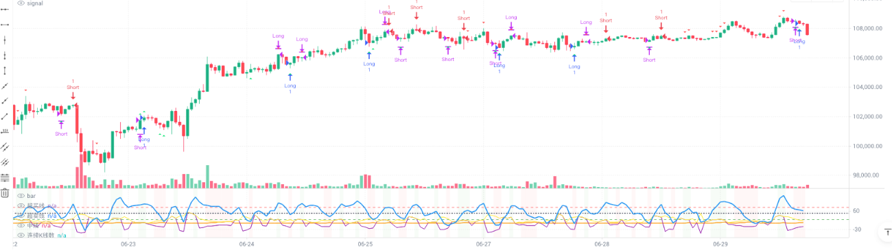
The results this time really surprised me. While it’s not a perfect strategy, it was clearly a big step up from the first version:
- Far fewer false signals, thanks to the continuity check filtering out a lot of noise
- Noticeable improvement in win rate
- Cleaner, more intuitive strategy logic
Looking at the equity curve in the backtest report gave me a strong sense of accomplishment. It might not be a groundbreaking strategy, but it came from a single idea that I explored and refined step by step.
Reflections on the Tools
This experience gave me a new appreciation for both the AI assistant and the quant platform itself.
The Value of the AI Assistant:
I used to think of AI as just a basic support tool — but now I realize how genuinely useful it can be in quantitative trading. Its greatest value isn’t replacing human thinking, but shortening the gap between an idea and working code dramatically.
- Strong comprehension – I used very simple language to describe my idea, and it was able to interpret it accurately and translate it into fully formed strategy logic
- Fast iteration – When I suggested improvements, it quickly pinpointed the issue and delivered a revised solution
- Solid code quality – The generated code ran smoothly, had clear structure, and included helpful comments
The Convenience of the Quant Platform:
I was also really impressed by the FMZ platform’s backtesting tools. In the past, backtesting a strategy meant hunting down historical data, building a custom backtest framework, and dealing with all sorts of technical hurdles. Now, I just paste in the code, set a few parameters, and get results instantly.
This kind of instant feedback made the whole exploration process feel seamless. Idea → Code → Validation → Refinement—it became a fast and smooth feedback loop.
Some Reflections
Of course, this journey also made me think more critically about a few things:
The Limitations of AI:
While the AI assistant was incredibly helpful, it’s not a magic bullet. The issues with the first version of the code weren’t something the AI could spot on its own — it still required human analysis and judgment. Even the suggestions it provides aren’t always optimal; they need to be adapted based on the actual trading context.
The Limitations of the Strategy Itself:
Even though the strategy performed well in backtests, it’s far from perfect. It doesn’t do particularly well in choppy or sideways markets, and the parameters need to be fine-tuned for different cryptocurrencies.
What’s more, just because a strategy works well on historical data doesn’t mean it will be effective in the future. Markets change, and strategies must evolve with them.
Unexpected Takeaways
Beyond the strategy itself, this whole experience brought me a few unexpected gains:
A New Perspective on Quant Trading:
I used to think quant trading had a very high barrier to entry—that it required strong programming skills and deep math knowledge. But this experience showed me that ideas and logic matter just as much. With the right tools, the technical barrier isn’t as high as I once believed.
A New Attitude Toward Learning:
In the past, whenever I came across an interesting idea, I’d tell myself, “I’ll try it when I have time.” More often than not, that time never came. But this experience showed me that today’s tools make it so easy to just try things. The only thing that really matters is having the courage to take action.
A Shift in How I View Failure:
When the first version of the strategy didn’t perform well, I didn’t give up. I dug in and tried to understand why. That process helped me realize that failure isn’t a dead end — it’s often a clue that leads you in the right direction.
What’s Next
The current version of the strategy is still sitting in my codebase, and I use it from time to time. It may not be perfect, but as the result of a personal exploration, I’m quite satisfied with it.
More importantly, this experience gave me confidence. The gap between an idea and a working strategy isn’t as wide as I used to think.
Going forward, I plan to keep exploring:
- Stay curious about trading theories and unconventional ideas
- Try applying concepts from other domains to trading
- Keep using AI and quant platforms to quickly test and validate ideas
Advice for Others
If you’re also interested in quantitative trading, here’s my advice:
- Don’t be intimidated by the tech – Today’s tools are incredibly powerful. What matters most is having ideas and the will to execute them.
- Start small – Don’t aim for the perfect strategy right away. Begin with simple ideas and build from there.
- Embrace trial and error – It’s normal to not get it right the first time. What’s important is to learn, adapt, and keep improving.
- Keep an open mind – Stay curious. Inspiration often comes from the most unexpected places.
Summary
Looking back, this whole journey started with just a single comment I saw on Bilibili—but it ended up leading me through an entire strategy development process.
In this age where knowledge and tools are more accessible than ever, maybe what we lack isn’t resources, but the courage to simply try. Whether you’re new to quant trading or already experienced, it’s worth starting from just one small idea and seeing where it takes you.
Who knows? Your next trading breakthrough might be hiding in a random comment you just scrolled past.
Disclaimer: This is a personal learning experience and not financial advice. Trading involves risk—please make decisions carefully.
From: When Top Comments Meet AI Quant: A Journey Into Strategy Implementation