Last week, when introducing How to Measure Position Risk - An Introduction to the VaR Method, it was mentioned that the risk of a portfolio is not equal to the risks of individual assets and is related to their price correlation. Taking two assets as an example, if their positive correlation is very strong, meaning they rise and fall together, then diversifying investments will not reduce risk. If there's a strong negative correlation, diversified investments can reduce risk significantly. The natural question then arises: how do we maximize returns at a certain level of risk when investing in a portfolio? This leads us to Markowitz Theory, which we are going to introduce today.

The Modern Portfolio Theory (MPT), proposed by Harry Markowitz in 1952, is a mathematical framework for portfolio selection. It aims to maximize expected returns by choosing different combinations of risk assets while controlling risk. The core idea is that the prices of assets do not move completely in sync with each other (i.e., there is incomplete correlation between assets), and overall investment risk can be reduced through diversified asset allocation.

The Key Concept of Markowitz Theory

1. Expected Return Rate: This is the return that investors expect to receive from holding assets or an investment portfolio, usually predicted based on historical return data.

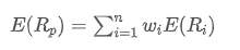
Where, 

 is the expected return of the portfolio, 

 is the weight of the i-th asset in the portfolio, 

 is the expected return of the i-th asset.

2. Risk (Volatility or Standard Deviation): Used to measure the uncertainty of investment returns or the volatility of investments.

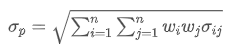
Where, 

 represents the total risk of the portfolio, 

 is the covariance of asset i and asset j, which measures the price change relationship between these two assets.

3. Covariance: Measures the mutual relationship between price changes of two assets.

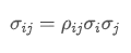
Where, 

 is the correlation coefficient of asset i and asset j, 

 and 

 are respectively the standard deviations of asset i and asset j.

4. Efficient Frontier: In the risk-return coordinate system, the efficient frontier is the set of investment portfolios that can provide the maximum expected return at a given level of risk.

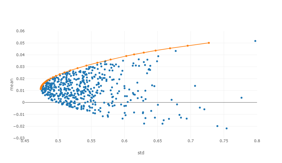
The diagram above is an illustration of an efficient frontier, where each point represents a different weighted investment portfolio. The x-axis denotes volatility, which equates to the level of risk, while the y-axis signifies return rate. Clearly, our focus lies on the upper edge of the graph as it achieves the highest returns at equivalent levels of risk.

In quantitative trading and portfolio management, applying these principles requires statistical analysis of historical data and using mathematical models to estimate expected returns, standard deviations and covariances for various assets. Then optimization techniques are used to find the best asset weight allocation. This process often involves complex mathematical operations and extensive computer processing - this is why quantitative analysis has become so important in modern finance. Next, we will illustrate how to optimize with specific Python examples.

Python Code Example for Finding the Optimal Combination Using Simulation Method

Calculating the Markowitz optimal portfolio is a multi-step process, involving several key steps, such as data preparation, portfolio simulation, and indicator calculation. Please refer to: https://plotly.com/python/v3/ipython-notebooks/markowitz-portfolio-optimization/

1. Obtain market data:

Through the get_data function, obtain the historical price data of the selected digital currency. This is the necessary data for calculating returns and risks, which are used to build investment portfolios and calculate Sharpe ratios.

2. Calculate Return Rate and Risk:

The calculate_returns_risk function was used to compute the annualized returns and annualized risk (standard deviation) for each digital currency. This is done to quantify the historical performance of each asset for use in an optimal portfolio.

3. Calculate Markowitz Optimal Portfolio:

The calculate_optimal_portfolio function was used to simulate multiple investment portfolios. In each simulation, asset weights were randomly generated and then the expected return and risk of the portfolio were calculated based on these weights.
By randomly generating combinations with different weights, it is possible to explore multiple potential investment portfolios in order to find the optimal one. This is one of the core ideas of Markowitz's portfolio theory.

The purpose of the entire process is to find the investment portfolio that yields the best expected returns at a given level of risk. By simulating multiple possible combinations, investors can better understand the performance of different configurations and choose the combination that best suits their investment goals and risk tolerance. This method helps optimize investment decisions, making investments more effective.

import numpy as np
import pandas as pd
import requests
import matplotlib.pyplot as plt

# Obtain market datadefget_data(symbols):
    data = []
    for symbol in symbols:
        url = 'https://api.binance.com/api/v3/klines?symbol=%s&interval=%s&limit=1000'%(symbol,'1d')
        res = requests.get(url)
        data.append([float(line[4]) for line in res.json()])
    return data

defcalculate_returns_risk(data):
    returns = []
    risks = []

    for d in data:
        daily_returns = np.diff(d) / d[:-1]
        annualized_return = np.mean(daily_returns) * 365
        annualized_volatility = np.std(daily_returns) * np.sqrt(365)

        returns.append(annualized_return)
        risks.append(annualized_volatility)

    return np.array(returns), np.array(risks)

# Calculate Markowitz Optimal Portfoliodefcalculate_optimal_portfolio(returns, risks):
    n_assets = len(returns)
    num_portfolios = 3000

    results = np.zeros((4, num_portfolios), dtype=object) 


    for i inrange(num_portfolios):
        weights = np.random.random(n_assets)
        weights /= np.sum(weights)

        portfolio_return = np.sum(returns * weights)
        portfolio_risk = np.sqrt(np.dot(weights.T, np.dot(np.cov(returns, rowvar=False), weights)))

        results[0, i] = portfolio_return
        results[1, i] = portfolio_risk
        results[2, i] = portfolio_return / portfolio_risk
        results[3, i] = list(weights) # Convert weights to a listreturn results

symbols = ['BTCUSDT','ETHUSDT', 'BNBUSDT','LINKUSDT','BCHUSDT','LTCUSDT']
data = get_data(symbols)

returns, risks = calculate_returns_risk(data)
optimal_portfolios = calculate_optimal_portfolio(returns, risks)

max_sharpe_idx = np.argmax(optimal_portfolios[2])
optimal_return = optimal_portfolios[0, max_sharpe_idx]
optimal_risk = optimal_portfolios[1, max_sharpe_idx]
optimal_weights = optimal_portfolios[3, max_sharpe_idx]

# Output resultsprint("Optimal combination:")
for i inrange(len(symbols)):
    print(f"{symbols[i]} Weight: {optimal_weights[i]:.4f}")

print(f"Expected return rate: {optimal_return:.4f}")
print(f"Expected risk (standard deviation): {optimal_risk:.4f}")
print(f"Sharpe ratio: {optimal_return / optimal_risk:.4f}")

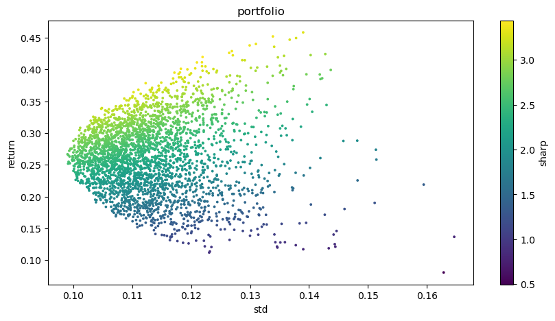
# Visualized investment portfolio
plt.figure(figsize=(10, 5))
plt.scatter(optimal_portfolios[1], optimal_portfolios[0], c=optimal_portfolios[2], marker='o', s=3)
plt.title('portfolio')
plt.xlabel('std')
plt.ylabel('return')
plt.colorbar(label='sharp')
plt.show()

Final output result:
Optimal combination:
Weight of BTCUSDT: 0.0721
Weight of ETHUSDT: 0.2704
Weight of BNBUSDT: 0.3646
Weight of LINKUSDT: 0.1892
Weight of BCHUSDT: 0.0829
Weight of LTCUSDT: 0.0209
Expected return rate: 0.4195
Expected risk (standard deviation): 0.1219
Sharpe ratio: 3.4403