In the previous article, we used quantitative analysis methods to screen currencies by amplitude and fluctuation preliminarily. Next, we will explore a key factor in grid trading – the setting of the number of grids. The number of grids determines the frequency of transactions and the amount of funds for each transaction, which in turn affects the total return and risk level of grid trading. Therefore, how to reasonably set the number of grids to achieve the best balance point is an important issue that every grid trader needs to consider.
Challenges in Grid Number Setting
- Too few grids: If the number of grids is set too small, the intervals between grids are large, which means that the price needs a large fluctuation to reach the next grid. Although the transaction amount of each grid is large, it can capture larger fluctuation profits, but due to fewer trading opportunities, some profits brought by smaller fluctuations may be missed. Therefore, the overall profitability may be lower than expected.
- Too many grids: When the number of grids is set too high, the price range of each grid is smaller, the trading opportunities increase, and buying and selling can be done more frequently. However, since the funds for each transaction are small, such strategies often require high-frequency transactions to make profits. This easily leads to higher handling fees, and too frequent transactions may make small market fluctuations the main source of profit, and the upper limit of profit is limited.
- Reasonable number of grids: The appropriate number of grids needs to take into account the volatility of the market, the size of the account funds, and the expected trading frequency. When the market volatility is large, increasing the number of grids appropriately can better capture the fluctuations, while when the funds are large, setting a smaller number of grids may bring a higher single transaction amount and reduce the pressure of handling fees. By balancing the grid spacing and the cost of frequent transactions, the benefits and risk control of the strategy can be maximized.
Basis for Setting the Number of Grids
1. Grid spacing and fund allocation
A core feature of grid trading is to allocate funds to each interval by setting multiple grid intervals. When determining the number of grids, we need to calculate the interval of each grid and the amount of funds in each grid first. The setting of the number of grids not only affects the amount of funds in each grid, but also determines the buying and selling price range of each grid.
- Grid spacing : When the grid is too dense, although there are more trading opportunities, the amount of funds for each transaction is smaller, which may lead to a lower upper limit on total returns; on the contrary, when the grid is too sparse, although the amount of funds for each transaction is larger, due to the low transaction frequency, profitable opportunities may be missed.
- Fund allocation : When setting the number of grids, we need to balance the fund allocation to avoid too much funds being dispersed in each grid and failing to obtain profits effectively.
2. Account funds and risk management
Account funds are an important factor in determining the number of grids. Larger account funds allow for more grids, while smaller account funds require a limit on the number of grids to avoid too much dispersion of funds, resulting in too little funds in each grid and inability to make a profit effectively.
In addition, the risk management strategy of grid trading also needs to take into account the setting of the number of grids. Especially when the market fluctuates violently, too many grids may lead to more losses, so the number of grids should be reasonably controlled to avoid over-trading.
Grid Trading Strategy Implementation
In the actual application of grid trading strategies, especially when optimizing the balance between the number of grids and the rate of return, the DQL (DATA Query Language) of the [Database] module provides great flexibility. DQL not only supports efficient data query, processing and analysis, but also helps traders simulate and backtest the performance of grid trading strategies in order to find the most suitable number of grids and other parameter configurations.
Through DQL, we can easily obtain historical K-line data from multiple exchanges (such as Binance) and adjust grid trading strategies based on this data. This allows us to screen out the optimal grid trading strategy accurately based on different market environments and the volatility of specific currencies.
1. Get the data
Before starting the backtest of the grid trading strategy, we first need to obtain the market data of the target currency. The following is the code to query the K-line data of the specified currency from the database:
# Get the K-line data of the target currency
data = query("select * from klines.spot_1d where Exchange = 'Binance' and Symbol = '???_usdt' order by Time")
Illustration:
- By querying the database, we can obtain the daily data (including time, opening price, highest price, lowest price and closing price, etc.) of a specific currency (such as
???_usdt) on the Binance trading platform. This provides basic data for strategy execution.
2. Grid strategy function
The core of the grid trading strategy is to trade using the preset grid quantity and price range. The specific steps are as follows:
1). Calculate the grid interval (gap) and the transaction amount per grid (notional) :
Grid interval (gap): calculated based on the ratio between the highest and lowest prices in the market. The formula is as follows:
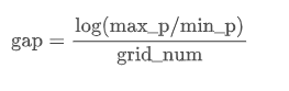
Among them, max_p is the highest price, min_p is the lowest price, and grid_num is the number of grids.
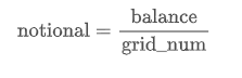
Nnotional : The notional of each grid is calculated by the total funds and the number of grids. The formula is:
2). Grid start and end prices:
The starting price and ending price of each grid are calculated dynamically based on the grid interval. For example, the first grid’s starting price is the lowest price, the second grid’s starting price is the lowest price multiplied by exp(gap), and so on.
3). Trading operations:
Opening condition : When the price drops to the starting price of a certain grid, a buy operation is executed.
Closing condition : When the price rises to the end price of a certain grid, a sell operation is executed.
4). Transaction fee : Assuming the handling fee for each transaction is 0.0001, we need to calculate and accumulate the handling fee for each transaction.
defgrid_trading_strategy(
    raw,
    grid_num,              # Grid number
    min_p,                # Lowest price
    max_p,                # Highest price
):
    """
    Functions for executing grid trading strategies
    """# Initializing variables
    balance = 1000# Initial capital
    raw = raw[['Time', 'Open', 'High', 'Low', 'Close']]  # Select only relevant columns# Setting up a grid trading strategy
    gap = math.log(max_p / min_p) / grid_num   # Calculate grid spacing
    notional = balance / grid_num            # Transaction volume per grid# Initialize the grid
    net = []
    for i inrange(grid_num):
        net.append({
            'start_p': min_p * math.exp(i * gap),   # Starting price for each grid'end_p': min_p * math.exp((i + 1) * gap),  # Ending price for each grid'amt': notional / (min_p * math.exp(i * gap)),  # Purchase quantity per grid'status': 'idle'# The initial state is idle
        })

    # Record status
    state = {
        'stock': 0,           # Current positions'fee': 0,             # Transaction fees'longTradeVol': 0,    # Long-term trading volume'shortTradeVol': 0,   # Short-term trading volume'profitTbl': [],      # Store the profit at each moment'feeTbl': [],         # Storage fees at each moment'netCnt': 0,          # Record net transactions'idx': 0# The index of the current data
    }

    # Check open tradesdefcheck_open_orders(state, net):
        for i inrange(len(net)):
            if net[i]['status'] == 'idle'and raw['Low'][state['idx']] <= net[i]['start_p'] and raw['Open'][state['idx']] > net[i]['start_p']:
                net[i]['status'] = 'taken'# Grid occupied
                tradeVol = net[i]['amt'] * net[i]['start_p']
                state['stock'] += net[i]['amt']
                state['longTradeVol'] += tradeVol
                state['fee'] += tradeVol * 0.0001# Assume the handling fee is 0.0001# Checking closed tradesdefcheck_close_orders(state, net):
        for i inrange(len(net)):
            if net[i]['status'] == 'taken'and raw['High'][state['idx']] >= net[i]['end_p'] and raw['Open'][state['idx']] < net[i]['end_p']:
                net[i]['status'] = 'idle'# The grid status returns to idle
                tradeVol = net[i]['amt'] * net[i]['end_p']
                state['stock'] -= net[i]['amt']
                state['shortTradeVol'] += tradeVol
                state['fee'] += tradeVol * 0.0001# Assume the handling fee is 0.0001
                state['netCnt'] += 1# Logging profits and expensesdeflog(state):
        addVol = state['stock'] * raw['Close'][state['idx']]  # The total value of the current position
        pl = state['shortTradeVol'] - state['longTradeVol'] + addVol  # Calculating profit
        state['profitTbl'].append(pl)
        state['feeTbl'].append(state['fee'])

    # Main trading loopfor i inrange(len(raw)):
        state['idx'] = i
        if raw['Close'][state['idx']] >= raw['Open'][state['idx']]:
            check_open_orders(state, net)
            check_close_orders(state, net)
        else:
            check_close_orders(state, net)
            check_open_orders(state, net)
        log(state)

    # Organize profit and expense data into a DataFrame
    pl = DataFrame({'pl' : state['profitTbl'],  'fee' : state['feeTbl']})
    pl['time'] = raw['Time']
    pl['pl-net'] = pl['pl'] - pl['fee']

    return pl
3. Backtesting
For the target currency, we choose the ‘oax_usdt’ currency. After the previous code test, this currency maintains a high amplitude for a long period of time without showing a significant unilateral trend. We can try to use different grid numbers (for example: 5, 10, 15, etc.) for simulated backtesting to see the effects of different grid numbers and find the appropriate grid number. For example, by calculating the net profit (pl-net) under each grid number, we can evaluate which grid numbers can bring the best returns in the current market environment. The following is the code for running the backtest:
grid_nums = [5*i+5for i inrange(5)]
out = []
for g in grid_nums:
    pl = grid_trading_strategy(
        data,
        grid_num=g,
        min_p=min(data['Close']),
        max_p=max(data['Close'])
    )
    out.append({
        'num': g,
        'pl-net': pl['pl-net'][-1],
        'min_pl': min(pl['pl-net']),
        'max_pl': max(pl['pl-net'])
    })

return out
4. Experimental results analysis
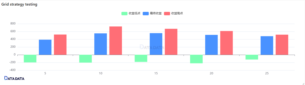
After backtesting with different grid number configurations, we obtained the following results:
Analysis:
- As the number of grids increases, the net profit increases first and then decreases. When the number of grids is 15, the net profit reaches the maximum value. As the number of grids continues to increase, the net profit decreases.
- The fluctuations of the minimum and maximum returns are similar to the trend of the net return, indicating that the choice of the grid number has an important impact on the return.
Summary
Reasonable setting of the number of grids is an important task in grid trading strategies. By optimizing the number of grids, the performance of grid trading strategies can be improved effectively and risks can be better controlled. This article analyzes the setting of the number of grids and provides specific calculation methods and sample codes, hoping to help you optimize grid trading strategies and improve the stability and profitability of the strategies.
Note:
The grid backtesting code in this article is adapted from the Zhihu veteran – Halcyon, for source code explanation, please refer to the article Algorithmic Trading Practice Diary (XVIII) – Details in grid trading: the relationship between the number of grids and long-term returns.
From: Quantitative Analysis Helps Grid Strategy (II): Relationship Between Grid Number and Yield