From a grid strategy that nearly blew up the account to a complete rewrite built together with AI
A grid running on the Korean equity market revealed four painful flaws in live trading. Following those four symptoms downward did not lead to another round of parameter tuning, but to an entirely new mathematical foundation. And throughout the whole process, the truly scarce ability was not “solving the problem,” but “asking the right question.”
- Instrument: EWY Korea equity index exposure (contract)
- Structure: Dynamically shifting grid, 10× leverage
- Final result: General-Purpose Grid Strategy · Mathematically Adaptive Edition v4.0
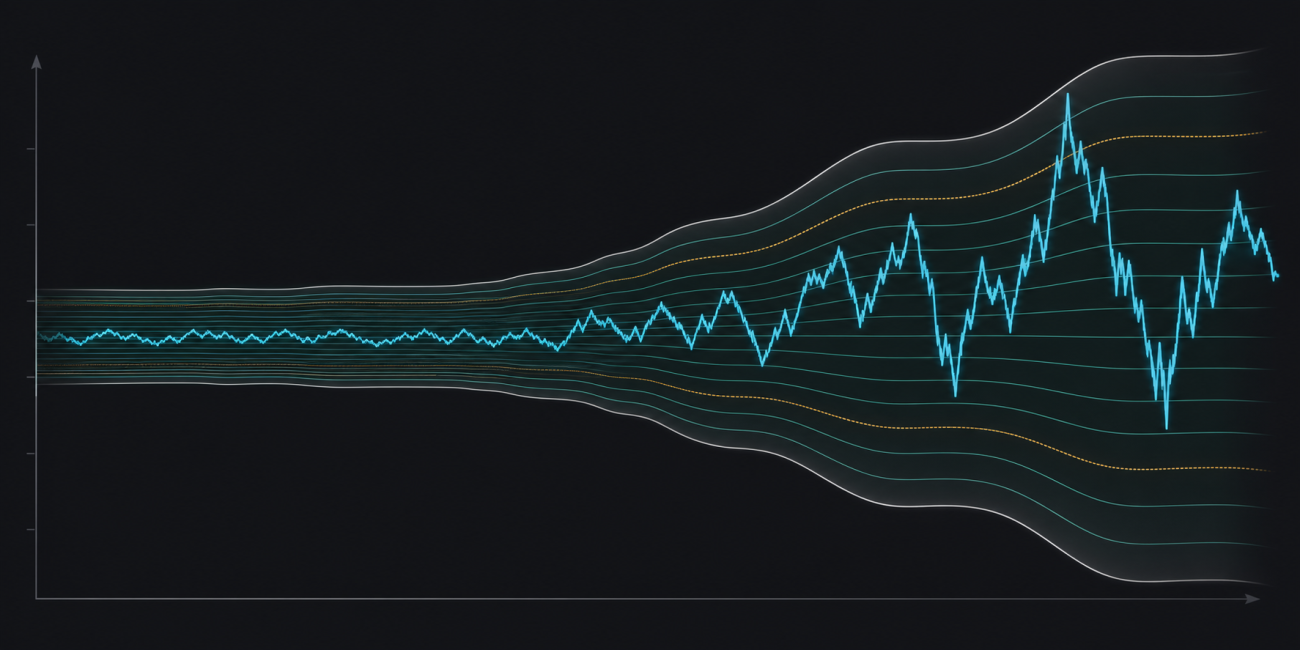
Figure 1: The fixed grid on the left keeps accumulating risk during a trend, while the adaptive structure on the right is supported by recursive estimators and risk-control gates.
00 · The Beginning: One Grid, Four Thorns
The story began with a discretionary view. I was bullish on a stretch of the Korean market, so I deployed a general-purpose grid on EWY: buy low and sell high inside a range, and shift the grid in the favorable direction after a breakout. The logic was clean, and the backtest looked good.
But once real money was involved, four problems began to surface, one after another. The following four sections describe what I genuinely felt while watching the strategy trade live.
Thorn 1 · Inefficiency. Both the grid spacing and the order size per level were hard-coded constants. But equities do not fluctuate uniformly around the clock. Between the Asian close and the U.S. open, price can barely move and volatility can become extremely low. Yet the grid was still using the same wide range and the same order size as during volatile periods. Orders sat sparsely across the range for hours without getting filled, while capital remained idle. Of course, when unexpected news arrived, volatility could suddenly explode. The problem was obvious: during low-volatility periods, the strategy was still placing orders across a fixed, wide range, making capital usage painfully inefficient.
Thorn 2 · Liquidation risk. This was the most dangerous flaw. Once the market entered a persistent decline, the long grid kept buying at lower and lower levels—buying more as price fell, accumulating a larger position, and doing so without any stop-loss. Under 10× leverage, this is the classic “catching a falling knife” pattern. Inventory keeps growing until liquidation becomes only a matter of time. The strategy could display the liquidation price, but it merely displayed it. It never intervened.
Thorn 3 · Giving back profits and wasting time while waiting. The grid slowly accumulated profits during sideways markets, and the equity curve looked attractive. But once there was a meaningful downward move, nearly all of those gains were given back. What came next was even worse: I was left holding a pile of trapped long positions and could do nothing but wait for price to revert before each one could exit at its take-profit level. That wait could last a long time. Capital remained locked, and the opportunity cost kept growing.
Thorn 4 · Dead inventory at the top. Positions opened at high prices were effectively being subsidized by repeated small profits harvested near the bottom. The strategy was slowly “grinding away” their losses through lower-range oscillations. The process was slow and passive. What I wanted was different: the grid’s upper boundary should be able to move down dynamically, instead of endlessly carrying expensive inventory opened near the top.
These four thorns looked like four separate defects. But once I dug deeper, they all turned out to be the same problem.

Figure 2: Small profits accumulate during the oscillating phase; once the market enters a one-way decline, the risk from counter-trend inventory expands at a much faster rate.
01 · Diagnosis: Four Symptoms, One Root Cause
The clearest way to explain it is with Greek letters. A grid is fundamentally a short-volatility or short-gamma strategy: it earns money from repeated back-and-forth movement and therefore depends on mean reversion. But a long grid keeps catching falling knives during a decline, causing its net position—its delta—to grow larger and larger. It has no defense against a persistent trend.
Decomposing the P&L gives the following structure:
Grid P&L  ≈  ( Oscillation Harvest ∝ σ²/d )  −  ( Inventory × Trend Drift μ )
              └── Always positive: earns from movement ──┘   └── Pure loss for a long book in a decline ──┘
- Oscillation term: The more frequently price crosses grid spacing
d, and the larger volatilityσbecomes, the more the strategy harvests. This term is always positive. - Trend term:
Inventory × μ. In a sustained decline,μremains negative while inventory keeps increasing. This term can diverge and eventually consume everything.
The real root cause: this was a short-volatility strategy with no meaningful risk control.
Worse still, the traditional grid design of “moving only in the favorable direction” is actually the opposite of the grid’s original purpose. When price breaks above the upper boundary, the grid moves upward and places new long orders at higher prices—buying after the rise. When price breaks below the lower boundary, it does nothing: no downward reset, no order cancellation, no stop-loss—just continued knife-catching. That design actively amplifies the trend term.
Looking back at the four thorns—inefficiency, liquidation, profit giveback, and dead inventory—they were simply different expressions of the same Inventory × μ problem at different stages. Once that became clear, the direction of the redesign was obvious: parameter tuning was not enough. This naked short-gamma grid needed a mathematical skeleton capable of reasoning about risk.
02 · A Grid That Breathes
The first problem to solve was the most intuitive one: inefficiency. The range width should not be a fixed percentage of price. It should follow the structure of volatility.
When volatility is low, the grid should automatically contract and harvest smaller movements more densely. When volatility expands, the grid should open up so that a single long wick does not sweep through the entire structure. It should inhale and exhale like a pair of lungs.

Figure 3: On the left, volatility is low, so both spacing and total range contract. On the right, volatility expands, and the grid widens with the equilibrium amplitude.
03 · The Fog of Direction: Milliseconds Are Noise; Drift Is the Enemy
The core of thorns two and three was direction detection.
Millisecond-level market jumps can look frightening, but those moves are precisely the noise that a grid is supposed to harvest. You do not need to predict them, and in practice you cannot. What matters is the slow variable hidden underneath the noise: drift, μ. Its relevant timescale is minutes to hours, not milliseconds.
Treating high-frequency price jumps as directional signals and repeatedly stopping out is the cognitive error behind many failed grid strategies. Making decisions from noise guarantees two failures at once: you waste the strategy’s expected return through frequent stop-outs, fees, and false positives, while still failing to avoid the real trend.
So the problem became: how can the strategy continuously sense μ without repeatedly stopping out and without stubbornly holding through a genuine trend?
That required a “second eye.”
04 · The Second Eye: Confirmation, Not Prediction
EWY represents Korean equities, and it has major constituent exposures such as Samsung Electronics and SK Hynix. The key shift in thinking was to stop betting on “who leads whom.” Lead-lag relationships are unstable and can be disrupted by geopolitics, Federal Reserve policy, and news flow.
Instead, the constituents can be used to confirm whether a decline is real. This requires synchronization, not predictive leadership.
Mathematically, each EWY return can be decomposed into two parts:
r_EWY  =  β · r_reference  +  ε
          └─ systematic ─┘    └─ idiosyncratic ─┘
           broad/fundamental     EWY-specific
           → genuine trend       → likely to revert
The decision rule then becomes straightforward:
| EWY is falling, while… | Interpretation | Action |
|---|---|---|
| The constituents are falling as well | Systematic = fundamentally driven = genuine trend | Avoid it / do not fight it |
| The constituents are barely moving | Idiosyncratic = EWY-specific noise | Likely to revert; keep harvesting with the grid |
Price alone cannot reveal this difference. Every bearish candle looks the same. Adding the constituent stocks as a second eye separates trend from noise—exactly the boundary I had been looking for between “short-term deviation” and “long-term regime change.”
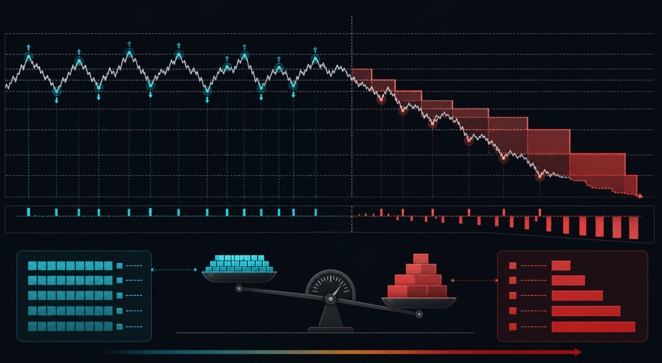
Figure 4: On the left, all three price streams weaken together, so the system identifies a broad trend and blocks counter-trend entries. On the right, only the target briefly deviates, so the mean-reversion channel remains active.
05 · Let the Parameters Converge on Their Own
There was another, deeper dissatisfaction: why should I decide the width of the range or how long the strategy should wait for reversion by intuition?
If the spread is mean-reverting, it can be modeled as an Ornstein–Uhlenbeck process. That means its timescale can be estimated from data instead of being entered manually as a parameter. The central quantity is the mean-reversion half-life:
H = ln(2) / θ (θ is the reversion speed)
- Half-life
Hdetermines the natural holding timescale. More importantly, it provides an exit criterion: if the spread still has not reverted afterk·H, the mean-reversion relationship may have deteriorated, confirming a regime shift. Exit instead of waiting forever. - Equilibrium amplitude
σ_eqdetermines the range width.
“How long is too long to wait?” changed from a subjective anxiety into a measurable number. For the first time, the wasted waiting described in thorn three had a precise gate.
06 · Convergence: Three Recursive Estimators
Every requirement eventually converged on one principle: recursive, online, and without a fixed lookback window.
Each new candle updates the state once. Memory adapts to the signal-to-noise ratio and the reversion speed instead of looking back over a fixed number of bars. Three estimators carry the entire decision framework.

Figure 5: The Kalman filter tracks local level and slope, RLS-OU estimates the reversion timescale, and cross-asset β decomposition isolates systematic drift. Together, the three outputs determine the range and the risk-control gates.
① Kalman Local Level + Slope — Replacing ATR, MA, and RSI
A two-dimensional Kalman filter—state = level + slope—tracks price online. It has no fixed lookback window. The Kalman gain adapts to the signal-to-noise ratio: memory becomes longer in stable conditions and shortens rapidly after structural change. Observation noise R, which functions as volatility, is estimated recursively online using Robbins–Monro adaptation. This is soft memory, not a fixed window.
def kf_step(st, y):
    """Kalman local level + trend; update one state dictionary point by point.
    Observation noise R adapts online with no fixed window.
    """
    st["price"] = y
    if not st["init"]:
        st["l"] = y
        st["s"] = 0.0
        st["R"] = max((y * 0.0005) ** 2, 1e-12)   # Initial volatility prior ≈ 5 bp
        st["init"] = True
        return

    R = st["R"] if st["R"] > 0 else 1e-12
    q_s = KF_Q_RATIO * R          # Slope process noise: responsiveness, the only soft prior
    q_l = KF_Q_RATIO * R * 0.25

    # Predict: F=[[1,1],[0,1]]
    l_pred = st["l"] + st["s"]
    s_pred = st["s"]
    pp00 = st["p00"] + st["p01"] + st["p10"] + st["p11"] + q_l
    pp01 = st["p01"] + st["p11"]
    pp10 = st["p10"] + st["p11"]
    pp11 = st["p11"] + q_s

    # Update: H=[1,0]
    e = y - l_pred                 # Innovation: current prediction error
    S = pp00 + R
    k0 = pp00 / S
    k1 = pp10 / S
    st["l"] = l_pred + k0 * e
    st["s"] = s_pred + k1 * e
    st["p00"] = (1 - k0) * pp00
    st["p01"] = (1 - k0) * pp01
    st["p10"] = pp10 - k1 * pp00
    st["p11"] = pp11 - k1 * pp01

    # Adaptive observation noise: Robbins–Monro soft memory, not a fixed window
    st["R"] = st["R"] + KF_ADAPT * (e * e - st["R"])
    st["sigma"] = math.sqrt(st["R"])                  # Instantaneous volatility
    st["z"] = st["s"] / (st["sigma"] + 1e-12)       # Trend strength = slope / volatility, signed
The output st["z"]—slope divided by volatility, a signed signal-to-noise measure per bar—is the trend-strength signal. Note that the state is stored in a dictionary called st: the same mathematical structure is reused for both the target and every reference instrument.
② RLS-AR(1) with a Self-Consistent Forgetting Factor — Letting the Timescale Emerge
Recursive least squares with a forgetting factor is used to fit:
price_t = a + b·price_{t-1}
The regression coefficient b is then converted into the OU half-life H and the equilibrium amplitude σ_eq.
The key idea is that the forgetting factor is itself determined by the estimated half-life. Memory is approximately OU_MEMORY half-lives long. In other words, the memory length converges from the data instead of being imposed as a manually chosen window.
def _rls_update(y_prev, y):
    """RLS-AR(1) estimator for mean reversion.
    The forgetting factor is determined self-consistently by the estimated half-life.
    No fixed window.
    """
    global _rls_a, _rls_b, _rls_p00, _rls_p01, _rls_p10, _rls_p11
    global _rls_resid_var, _rls_init, _ou_half_life, _ou_sigma_eq

    # Forgetting factor: memory ≈ OU_MEMORY half-lives.
    # Use a gentle default while the half-life is unknown.
    if _ou_half_life > 0:
        mem = max(OU_MEMORY * _ou_half_life, 5.0)
        ff = math.exp(-1.0 / mem)
    else:
        ff = 0.99
    ff = min(max(ff, 0.90), 0.9995)

    phi0, phi1 = 1.0, y_prev
    pph0 = _rls_p00 * phi0 + _rls_p01 * phi1
    pph1 = _rls_p10 * phi0 + _rls_p11 * phi1
    denom = ff + phi0 * pph0 + phi1 * pph1
    k0 = pph0 / denom
    k1 = pph1 / denom
    e = y - (_rls_a * phi0 + _rls_b * phi1)
    _rls_a += k0 * e
    _rls_b += k1 * e
    _rls_p00 = (_rls_p00 - k0 * pph0) / ff
    _rls_p01 = (_rls_p01 - k0 * pph1) / ff
    _rls_p10 = (_rls_p10 - k1 * pph0) / ff
    _rls_p11 = (_rls_p11 - k1 * pph1) / ff
    _rls_resid_var = _rls_resid_var + KF_ADAPT * (e * e - _rls_resid_var)

    b = _rls_b
    if 0.0 < b < 1.0:
        theta = -math.log(b)
        _ou_half_life = math.log(2.0) / theta               # Half-life in bars
        if (1 - b * b) > 1e-9 and _rls_resid_var > 0:
            _ou_sigma_eq = math.sqrt(
                _rls_resid_var / (1 - b * b)
            )                                              # Equilibrium amplitude
    else:
        _ou_half_life = 0.0   # b ≥ 1: no reversion (unit root/trend); handled by the trend gate
The range width is then determined directly by σ_eq. It adapts to volatility and reversion speed while remaining protected by upper and lower bounds—with no fixed lookback window:
def effective_width_abs(ref_price):
    """Set range width from OU equilibrium amplitude σ_eq.
    Adapt to the volatility structure; fall back to a fixed percentage before warm-up.
    """
    if estimators_ready() and _ou_sigma_eq > 0:
        w = WIDTH_SIGMA_MULT * _ou_sigma_eq
        floor_w = pct_to_abs(GRID_WIDTH_PCT, ref_price) * WIDTH_FLOOR_FRAC
        cap_w = pct_to_abs(GRID_WIDTH_PCT, ref_price) * WIDTH_CAP_MULT
        return min(max(w, floor_w), cap_w)
    return pct_to_abs(GRID_WIDTH_PCT, ref_price)
③ Cross-Asset β Decomposition + Inventory Risk Control — The Second Eye and the Seat Belt
This is where confirmation of a systematic trend is embedded into the strategy itself. For every new candle, the system recursively estimates the target’s regression coefficient β_j against each reference instrument in return space using EWMA. It then decomposes target drift into systematic and idiosyncratic components:
# Inside update_estimators: update β and systematic trend one bar at a time

# Recursive regression coefficient β_j = covariance / variance
# Soft memory with no fixed window
r_t = (c - prev_close) / prev_close            # Target return for the current bar
r_j = (rc - _ref_prevc[j]) / _ref_prevc[j]     # Reference return for the current bar
_ref_cov[j] += KF_ADAPT * (r_t * r_j - _ref_cov[j])
_ref_var[j] += KF_ADAPT * (r_j * r_j - _ref_var[j])
_ref_beta[j] = _ref_cov[j] / _ref_var[j]

# Systematic drift confirmed by the references:
# ĝ_sys = Σ β_j · reference fractional drift
g_sys = 0.0
for j in range(nref):
    g_sys += _ref_beta[j] * (_kf_refs[j]["s"] / _kf_refs[j]["price"])
sig_frac = _vol_sigma / pt
_trend_z_sys = g_sys / (sig_frac + 1e-12)       # Systematic trend strength
_sys_share = abs(g_sys) / (abs(g_t) + 1e-12)    # Systematic share
The trend gate therefore responds only to the component confirmed by the references. When reference instruments are enabled, it uses systematic z_sys; otherwise, it falls back to the target’s own z:
def gate_trend_z():
    """
    References enabled and data available:
        use systematic z_sys, the component confirmed by Samsung, SK Hynix, and others.
    Otherwise:
        fall back to the target's own z.

    Target falls but references do not:
        idiosyncratic noise, z_sys ≈ 0, so the grid keeps harvesting.
    Target and references fall together:
        genuine systematic trend, z_sys becomes significant, so counter-trend entries are blocked.
    """
    if ref_n() > 0 and _refs_ok and estimators_ready():
        return _trend_z_sys
    return _trend_z
The “flexible lowering of the upper boundary” from thorn four is implemented through an inventory reservation-price adjustment, a discrete version of the Avellaneda–Stoikov reservation price. The larger the long inventory becomes, the more the effective upper boundary is pushed downward. New long entries at high prices automatically stop—the ceiling lowers itself.
def effective_ceiling():
    """As long inventory grows, push the effective upper boundary downward.
    Stop adding at high prices and let the ceiling adjust automatically.
    """
    long_amt = assets[base_currency].get("long_amount", 0)
    short_amt = assets[base_currency].get("short_amount", 0)
    net_usdt = (
        (long_amt - short_amt)
        * assets[base_currency]["ctVal"]
        * get_price()
    )
    inv_ratio = min(
        max(0.0, net_usdt / (Funding * MAX_NET_EXPOSURE_MULT)),
        1.0,
    )
    drop = INVENTORY_SKEW * inv_ratio * (range_high - range_low)
    return range_high - drop
All gates are unified inside the entry decision: trend, hard net-exposure limit, inventory ceiling, and drawdown circuit breaker. If any one of them fails, no new position is opened. Existing take-profit orders are never force-closed. In other words, the strategy neither adds aggressively against the trend nor stops out repeatedly.
def can_open(side, grid_price):
    """Mathematical gates for new entries:
    trend / net exposure / inventory ceiling / drawdown breaker.
    """
    if estimators_ready():
        gz = gate_trend_z()
        if side == "long" and gz <= -TREND_Z_THRESHOLD:
            return False, "trend"
        if side == "short" and gz >= TREND_Z_THRESHOLD:
            return False, "trend"

    # Hard cap on net exposure: prevent unlimited falling-knife accumulation
    net_usdt = (long_amt - short_amt) * ct_val * price
    if side == "long" and net_usdt >= Funding * MAX_NET_EXPOSURE_MULT:
        return False, "risk"
    if side == "short" and -net_usdt >= Funding * MAX_NET_EXPOSURE_MULT:
        return False, "risk"

    # Inventory ceiling: stop opening new longs at high prices
    if side == "long" and grid_price > effective_ceiling():
        return False, "skew"

    if check_drawdown_breaker():
        return False, "dd"
    return True, ""
07 · Implementation: Removing All Four Thorns at Once
After the strategy was rebuilt as v4.0, each thorn mapped directly to a mathematical mechanism. These were no longer isolated patches, but different projections of the same underlying framework:
| Live-Trading Problem | Mathematical Mechanism |
|---|---|
| Inefficiency in low volatility | Range width = WIDTH_SIGMA_MULT · σ_eq, breathing adaptively with the volatility structure |
| Liquidation risk during declines | Kalman trend gate blocks counter-trend entries + hard cap on net exposure |
| Profit giveback / endless waiting | No counter-trend accumulation + half-life-based exit criterion + drawdown circuit breaker |
| Dead inventory at high prices | Inventory reservation-price shift → effective upper boundary falls as long inventory accumulates |
The reference contracts only need to be entered as one parameter line:
SAMSUNG_USDT, SKHYNIX_USDT
The strategy reads them directly through GetRecords, with no need to configure additional exchanges. Everything else adapts automatically.
08 · Validation: The Second Eye Opens
The framework was validated numerically using synthetic sequences. EWY was declining in both cases, but the gate produced opposite actions depending on whether the constituent references confirmed the move. That is exactly what “confirmation rather than prediction” should look like:
| Scenario | Target z | Systematic z | β | Systematic Share | Action |
|---|---|---|---|---|---|
| References fall together with EWY (genuine trend) | −0.324 | −0.281 | +0.81 | 87% | 🚫 Block counter-trend longs |
| References do not move (idiosyncratic noise) | −0.269 | +0.027 | −0.38 | 10% | ✅ Keep harvesting |
Looking only at the target, both cases appear bearish (z ≈ −0.3). But with the second eye, one is classified as a genuine decline to avoid, while the other is treated as noise to harvest. The distinction that price alone cannot reveal is extracted by the mathematics.
Epilogue
The real gain from this optimization was not the code. It was the path:
Start from a specific pain observed in live trading. Refuse to cover it with outdated rules that cannot justify themselves. Keep asking questions until the problem reaches first principles, and let the parameters converge from the data.
The four thorns eventually collapsed into two adjustable controls—trend sensitivity and range looseness—plus one risk preference. Everything else is left to the data, and to the backtest that must determine whether the foundation actually makes money.
That is the next part of the story.
Final Note · The Answer for This Era
To be honest, I do not fully understand all the mathematics in this article. I cannot derive the Kalman filter from first principles, clearly explain why the RLS forgetting factor should be self-consistent in exactly this way, or walk through the stochastic differential equation behind the OU half-life from beginning to end.
But that is precisely what makes this era so powerful.
To cook a good meal, we do not need to brew the soy sauce and vinegar ourselves. We can still create something delicious. In the age of large language models, the division of capability has quietly shifted: what matters most is no longer “solving problems,” but “discovering problems through practice.”
Tools can complete the solution path for us: derivation, modeling, coding, and validation. But the questions “Where does it hurt?”, “Why does it hurt?”, and “What is the real problem?” can only come from real practice.
I knew where to ask because I spent day after day watching those four thorns appear on the screen. I arrived at a recursive, windowless architecture because I kept insisting that fixed-window indicators were not good enough. Tools can answer questions, but they cannot decide which questions matter. They can complete the journey, but they cannot choose the direction.
The ladder of knowledge is becoming lower. Almost anyone can use tools to stand one step away from an answer. But precisely because answers are becoming easier to obtain, scarcity has shifted elsewhere: to the ability to see the real problem, and to the judgment required to choose the right path among countless surface-level explanations.
Choose the right direction, and the answer will eventually emerge. Choose the wrong direction, and greater computing power will only take you toward the wrong destination faster.
So this article is less a record of one quantitative strategy than a demonstration:
Someone who does not fully master every piece of the mathematics can still use the tools of this era to remove the problems one by one—as long as they can identify the four thorns precisely in live trading and refuse to settle for a plausible-sounding but superficial fix.
In an era when everyone can obtain answers, learn to ask the right questions first.