PINE Language Introductory Tutorial of FMZ Quant

FMZ Quant Trading Platform supports Pine language writing strategies, backtesting, and real bot running for Pine language strategies, and it is compatible with lower versions of Pine language. There are many Pine strategies (scripts) collected and transplanted in the Strategy Square on the FMZ Quant Trading Platform (FMZ.COM).

FMZ supports not only the Pine language, but also the powerful drawing function of the Pine language. Various functions, rich and practical tools, efficient and convenient management on the FMZ platform further enhance the practicability of the Pine strategy (script). Based on the compatibility with the Pine language, FMZ also expands, optimizes and trims the Pine language to a certain extent. Before entering the tutorial officially, let's take a look at the changes to the Pine language on FMZ and the original one.

A brief overview of some of the obvious differences:

1. The Pine strategy on FMZ, the version identifier at the beginning of the code //@version and the strategy, indicator statements at the beginning of the code are not mandatory to write, FMZ does not support import to import library function for now. It may be seen that some strategies written like this:

  //@version=5
  indicator("My Script", overlay = true)
  src = close
  a = ta.sma(src, 5)
  b = ta.sma(src, 50)
  c = ta.cross(a, b)
  plot(a, color = color.blue)
  plot(b, color = color.black)
  plotshape(c, color = color.red)

Or write it like this:

  //@version=5
  strategy("My Strategy", overlay=true)

  longCondition = ta.crossover(ta.sma(close, 14), ta.sma(close, 28))
  if (longCondition)
      strategy.entry("My Long Entry Id", strategy.long)

  shortCondition = ta.crossunder(ta.sma(close, 14), ta.sma(close, 28))
  if (shortCondition)
      strategy.entry("My Short Entry Id", strategy.short)

On FMZ it can be simplified to:

  src = close
  a = ta.sma(src, 5)
  b = ta.sma(src, 50)
  c = ta.cross(a, b)
  plot(a, color = color.blue, overlay=true)
  plot(b, color = color.black, overlay=true)
  plotshape(c, color = color.red, overlay=true)

Or:

  longCondition = ta.crossover(ta.sma(close, 14), ta.sma(close, 28))
  if (longCondition)
      strategy.entry("My Long Entry Id", strategy.long)

  shortCondition = ta.crossunder(ta.sma(close, 14), ta.sma(close, 28))
  if (shortCondition)
      strategy.entry("My Short Entry Id", strategy.short)

2. Some trading-related settings of the strategy (script) are set by the "Pine Language Trading Class Library" parameters on the FMZ strategy interface.
Closing price model and real-time price model
On the trading view, we can use the calc_on_every_tick parameter of the strategy function to set the strategy script to execute the strategy logic in real time when the price changes everytime. At this time, the calc_on_every_tick parameter should be set to true. The calc_on_every_tick default parameter is false, that is, the strategy logic is executed only when the current K-line BAR of the strategy is completely completed.
On FMZ, it is set by the parameters of the "Pine Language Trading Class Library" template.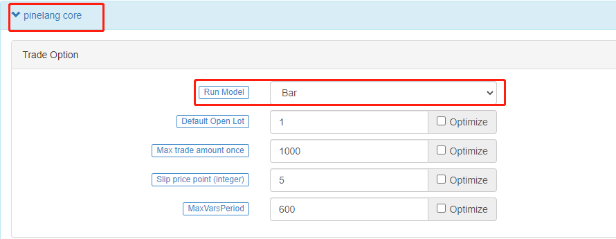
Numerical precision control such as price and order amount when the strategy is executed needs to be specified on FMZ
On trading view there is no accuracy problem when placing real bot orders because it can only be tested in simulation. On FMZ, it is possible to run the Pine strategy in real time. Then the strategy needs to be able to specify the price accuracy and order amount accuracy of the trading variety flexibly. The accuracy settings control the number of decimal places in the relevant data to prevent the data from not meeting the exchange's order requirements and thus failing to place an order.
Futures contract code
If the trading product on FMZ is a contract, it has two attributes, they are "Trading Pair" and "Contract Code" respectively. In addition to setting the trading pair explicitly, it is also necessary to set the specific contract code in the parameter "Variety Code" of the "Pine Language Trading Class Library" template during the real bot and backtesting. For example, for a perpetual contract, fill in swap, and the contract code depends on whether the operating exchange has such a contract. For example, some exchanges have quarterly contracts, you can fill in quarter here. These contract codes are consistent with the futures contract codes defined in FMZ's Javascript/python/c++ language API document. For other settings, such as the minimum order amount, default order amount, etc., please refer to the parameter introduction on ["Pine language trading library"] in the Pine language documentation (https://www.fmz.com/bbs-topic/9315#pine%E8 %AF%AD%E8%A8%80%E4%BA%A4%E6%98%93%E7%B1%BB%E5%BA%93%E6%A8%A1%E7%89%88%E5%8F %82%E6%95%B0).
3. Functions for FMZ extensions: runtime.debug , runtime.log, runtime.error used for debugging. 3 functions have been added to the FMZ platform for debugging.
runtime.debug: Print variable information on the console, which is generally not used with this function.
runtime.log: output in the log. PINE language-specific functions on FMZ. runtime.log(1, 2, 3, close, high, ...), Multiple parameters can be passed.
runtime.error: It will result in a runtime error with the error message specified in the message parameter when called. runtime.error(message)
4. The overlay parameter is extended in some of the drawing functions In the Pine language on FMZ, the drawing functions plot, plotshape, plotchar, etc. have added the overlay parameter support, allowing to specify the drawing on the main chart or sub-chart. overlay is set to true to draw on the main chart, and false is set to draw on the sub-chart, which enables the Pine strategy on FMZ to draw the main chart and the sub-chart at the same time.
5. syminfo.mintick value of built-in variables The built-in variable of syminfo.mintick is defined as the minimum tick value of the current species. This value can be controlled by the template parameter pricing currency precision in the "Pine Language Trading Class Library" on the FMZ bot/backtest interface. Pricing currency accurancy setting 2 means that the price is accurate to the second decimal place when trading, and the minimum price change unit is 0.01. The value of syminfo.mintick is 0.01.
6. The average prices in FMZ PINE Script are all inclusive of commission For example: the order price is 8000, the selling direction, the quantity is 1 lot (piece, sheet), the average price after the transaction is not 8000, but lower than 8000 (the cost includes the handling fee).

Pine language foundation

When starting to learn the basics of the Pine language, there may be some examples of instructions and code grammar that we are not familiar with. It doesn't matter if you don't understand it, we can familiarize yourself with the concepts first and understand the purpose of the test, or you can check the Pine language documentation on FMZ for instructions. Then follow the tutorial step by step to familiarize yourself with various grammars, instructions, functions, and built-in variables.

Model execution

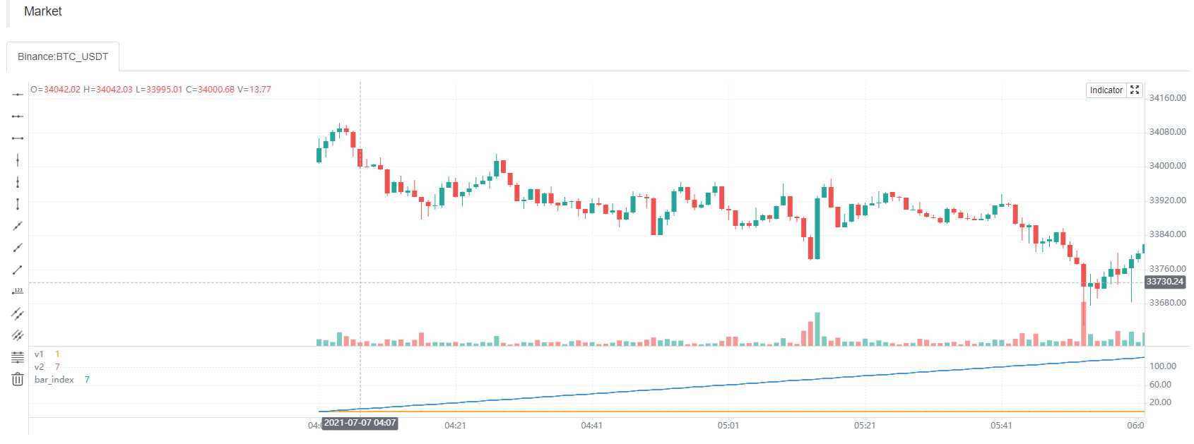
When starting to learn the Pine language, it is very necessary to understand the related concepts such as the execution process of the Pine language script program. The Pine language strategy runs based on the chart. It can be understood that the Pine language strategy is a series of calculations and operations, which are executed on the chart in the order of time series from the earliest data that has been loaded on the chart. The amount of data that the chart initially loads is limited. In the real bot, the maximum amount of the data is usually determined based on the maximum data volume returned by the exchange interface, and the maximum amount of the data during backtesting is determined based on the data provided by the data source of the backtesting system. The leftmost K-line Bar on the chart, that is, the first data of the chart data set, has an index value of 0. The index value of the current K-line Bar when the Pine script is executed can be referenced through the built-in variable bar_index in the Pine language.

plot(bar_index, "bar_index")

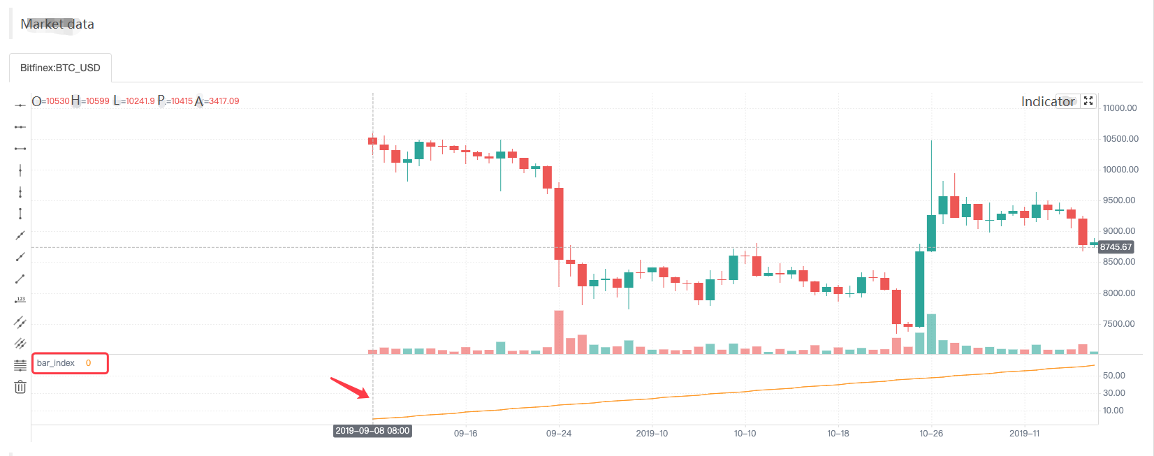
The plot function is one of the functions we will use more in the future. The use is very simple, it is to draw a line on the chart according to the passed parameters, the passed data is bar_index, and the line is named as bar_index. It can be seen that the value of the line named bar_index on the first Bar is 0, and it increases by 1 to the right as the Bar increases.

Because the settings of the strategy are different, the model execution methods of the strategy are different, they can be divided into closing price model and real-time price model. We have also briefly introduced the concepts of them before.

Closing price model When the strategy code is executed, the period of the current K-line Bar is completely executed, and when the K-line is closed, the K-line period has been completed. At this point, the Pine strategy logic is executed once, and the triggered trading signal will be executed at the beginning of the next K-line Bar.
Real-time price model When the strategy code is executed, regardless of whether the current K-line Bar is closed or not, the Pine strategy logic will be executed when the market changes every time, and the triggered trading signal will be executed immediately.

When the Pine language strategy is executed from left to right on the chart, the K-line Bars on the chart are divided into History Bar and Real-time Bar:

History Bar When the strategy is set to "Real bot price model" and starts to execute, all K-line Bars on the chart except the rightmost one are History Bar. The strategy logic is executed only once on each history bar.
When the strategy is set to "Close price model" and starts to execute, all bars on the chart are historical bars. The strategy logic is executed only once on each history bar. Calculation based on historical Bar:
The strategy code is executed once in the closing state of the historical bar, and then the strategy code continues to be executed in the next historical bar until all historical bars are executed once.
Real-time Bar When the strategy is executed to the last K-line Bar on the far right, the Bar is a real-time Bar. When the real-time bar is closed, the bar becomes a passing real-time bar (becomes a historical bar). A new real-time Bar will be generated at the far right of the chart. When the strategy is set to "real-time price model" and starts to execute, the strategy logic will be executed once for each market change on the real-time bar.
When the strategy is set to "close price model" and starts to execute, the real-time bar will not be displayed on the chart. Calculation based on real-time Bar:
If the strategy is set to "close price model" and the chart does not display the real-time bar, the strategy code will only be executed once when the current bar closes.
If the strategy is set to "real price model", the calculation on the real-time bar is completely different from the historical bar, and the strategy code will be executed once for each market change on the real bot bar. For example, the built-in variables high, low, close are determined on the historical Bar, and these values may change every time when the market changes on the real-time Bar. Therefore, data such as indicators calculated based on these values will also change in real time. On the real-time Bar, close always represents the current latest price, and high and low always represent the highest point and lowest point reached since the start of the current real-time bar. These built-in variables represent the final value of the real-time Bar when it was last updated. Rollback mechanism when executing strategies on real-time Bar (real-time price model):
During real-time Bar execution, resetting user-defined variables before each new iteration of the strategy is called rollback. Let's understand the rollback mechanism with an example of the following test code. Attention:

  /*backtest 
  ...
  ..
  .
  */

The content of the package is the backtest configuration information saved in the form of code on the FMZ platform.

  /*backtest
  start: 2022-06-03 09:00:00
  end: 2022-06-08 15:00:00
  period: 1m
  basePeriod: 1m
  exchanges: [{"eid":"Bitfinex","currency":"BTC_USD"}]
  */

  var n = 0
  if not barstate.ishistory
      runtime.log("before n + 1, n:", n, " current bar_index:", bar_index)
      n := n + 1
      runtime.log("after n + 1, n:", n, " current bar_index:", bar_index)

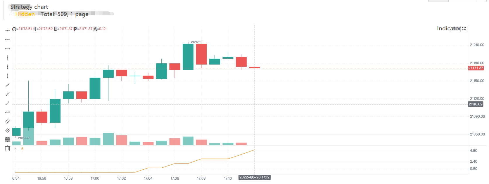
  plot(n, title="n")

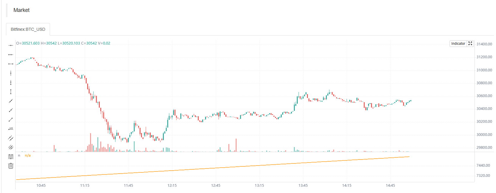
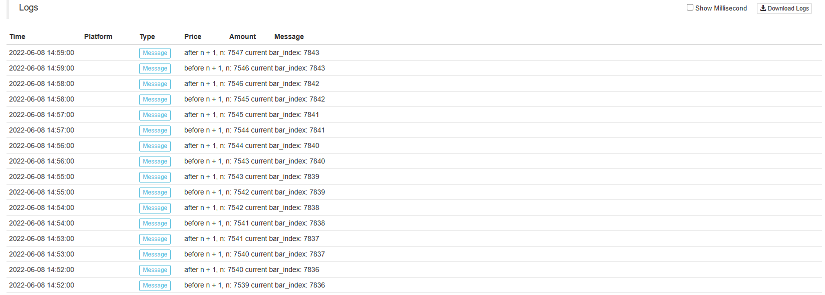
We only examine the scene executed in the real-time Bar, so we use the not barstate.ishistory expression to limit the accumulation of the variable n only in the real-time Bar, and use runtime.log function to output the information in the strategy log before and after the accumulation operation. From the curve n drawn using the drawing function plot, it can be seen that n is always 0 when the strategy is running in the history Bar. When the real-time Bar is executed, the operation of adding 1 to n is triggered, and the operation of adding 1 to n is executed when the strategy is executed in each round of the real-time Bar. It can be observed from the log message that n will be reset to the value finally submitted by the previous Bar execution strategy when the strategy code is re-executed in each round. The n value update will be submitted when the strategy code is executed on the real-time Bar for the last time, so you can see that the value of curve n increases by 1 with each increase of Bar starting from the real-time Bar on the chart.

Summary:

The strategy code is executed once every time the market is updated when the strategy starts executing in a real-time Bar.
When executed in a real-time Bar, the variables are rolled back each time before the strategy code is executed.
When executed in a real-time Bar, the variables are committed once when the close is updated. Due to the data rollback, drawing operations such as curves on the chart may also cause redrawing. For example, let's modify the test code just now and test it on a real bot:

  var n = 0
  if not barstate.ishistory
      runtime.log("before n + 1, n:", n, " current bar_index:", bar_index)
      n := open > close ? n + 1 : n
      runtime.log("after n + 1, n:", n, " current bar_index:", bar_index)

  plot(n, title="n")

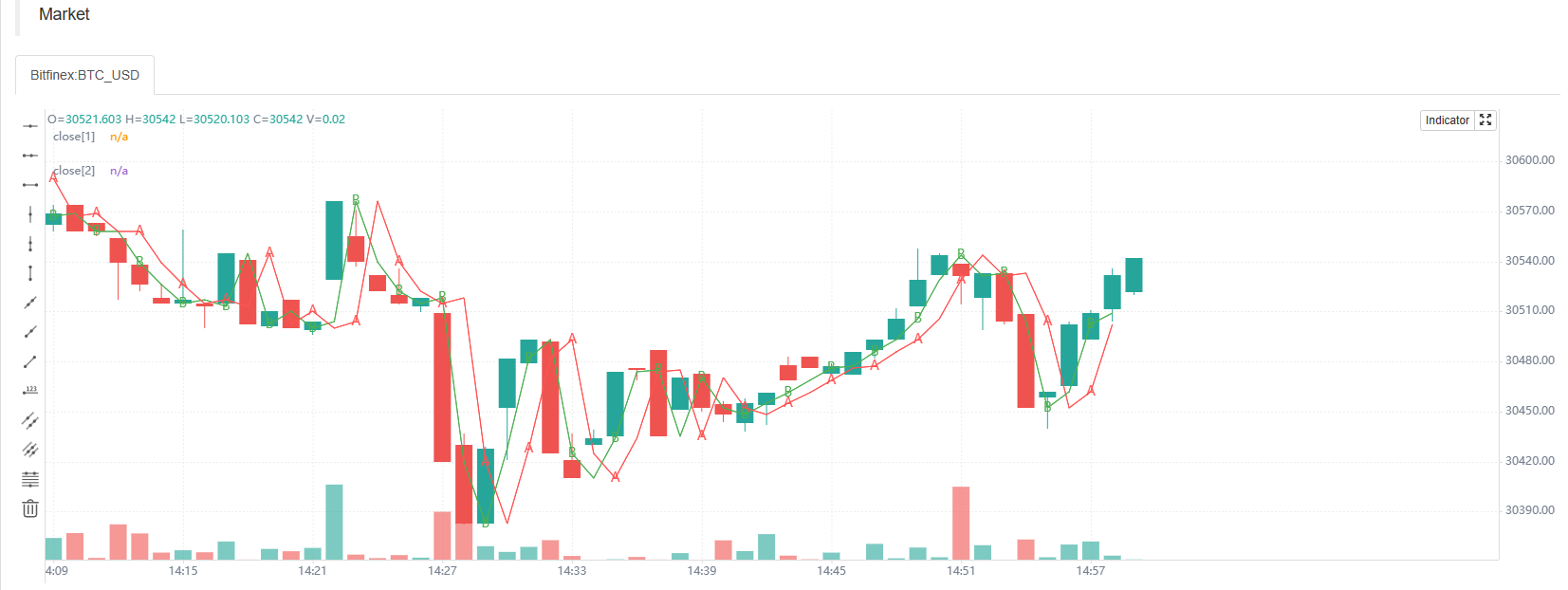
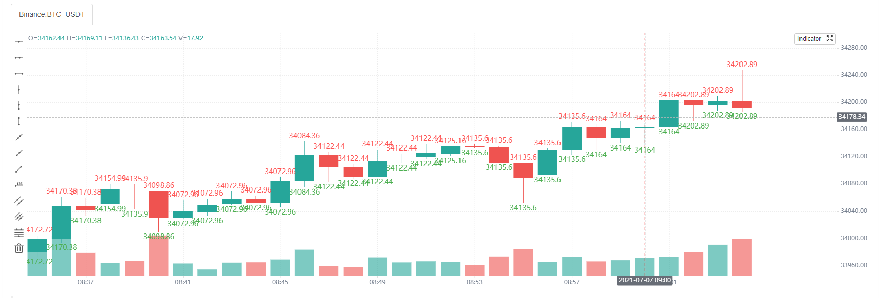
Screenshot of time A

Screenshot of time B

We only modified this sentence: n := open > close ? n + 1 : n, only add 1 to n when the current real-time Bar is a negative line (that is, the opening price is higher than the closing price). It can be seen that in the first chart (time A), since the opening price was higher than the closing price (negative line) at that time, n was accumulated by 1, and the value of n displayed on the chart curve was 5. Then the market changed and the price updated as shown in the second graph (time B). At this time, the opening price is lower than the closing price (positive line), and the n value rolls back and does not accumulate 1. The curve n in the chart is also redrawn immediately, and the value of n on the curve is 4. Therefore, the signals such as golden forks and dead forks displayed on the real-time bar are uncertain and may change.

Variable context in functions Let's study the variables in the Pine language function together. According to some descriptions on Pine tutorials, the variables in the function have the following differences from the variables outside the function:

The history of series variables used in the Pine function is created with each successive call to the function. If the function is not called on every bar on which the script runs, this will result in a discrepancy between the historical values of the series inside and outside the function's local block. Therefore, if the function is not called on each bar, the series referenced inside and outside the function with the same index value will not refer to the same historical point.

Is it a little hard to understand? Nevermind, we will figure it out with a test code running on FMZ:

  /*backtest
  start: 2022-06-03 09:00:00
  end: 2022-06-08 15:00:00
  period: 1m
  basePeriod: 1m
  exchanges: [{"eid":"Bitfinex","currency":"BTC_USD"}]
  */

  f(a) => a[1]
  f2() => close[1]  

  oneBarInTwo = bar_index % 2 == 0
  plotchar(oneBarInTwo ? f(close) : na, title = "f(close)", color = color.red, location = location.absolute, style = shape.xcross, overlay = true, char = "A")   
  plotchar(oneBarInTwo ? f2() : na, title = "f2()", color = color.green, location = location.absolute, style = shape.circle, overlay = true, char = "B")   
  plot(close[2], title = "close[2]", color = color.red, overlay = true)
  plot(close[1], title = "close[1]", color = color.green, overlay = true)

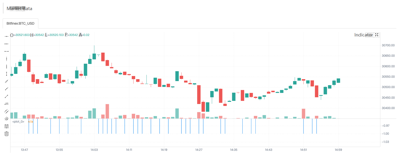
Screenshot of backtest running

The test code is relatively simple, mainly to examine the data referenced in two ways, namely: f(a) => a[1] and f2() => close[1] .

f(a) => a[1]: Use the method of passing parameters, the function returns to a[1] finally.
f2() => close[1]: Use the built-in variable close directly, and the function returns to close[1] finally. The [] symbol is used to refer to the historical value of the data series variable, and close[1] refers to the closing price data on the Bar before the current closing price. Our test code draws a total of 4 types of data on the chart:
plotchar(oneBarInTwo ? f(close) : na, title = "f(close)", color = color.red, location = location.absolute, style = shape.xcross, overlay = true, char = "A")
Draw a character "A", the color is red, it is drawn when oneBarInTwo is true, and the drawn position (on the Y axis) is: the returned value of f(close).
plotchar(oneBarInTwo ? f2() : na, title = "f2()", color = color.green, location = location.absolute, style = shape.circle, overlay = true, char = "B")
Draw a character "B", the color is green, it is drawn only when oneBarInTwo is true, and the drawn position (on the Y axis) is: the returned value of f2().
plot(close[2], title = "close[2]", color = color.red, overlay = true)
Draw a line, the color is red, and the drawn position (on the Y axis) is: close[2], which is the closing price of the second bar before the current bar (two bars from the left).
plot(close[1], title = "close[1]", color = color.green, overlay = true)
Draw a line, the color is green, and the drawn position (on the Y-axis) is: close[1], which is the closing price of the first bar before the current bar (one bar from the left). It can be seen from the screenshot of the strategy backtesting that although both the function f(a) => a[1] used to draw the A marker and the function f2() => close[1] use [1] to refer to the historical data on the data series, but the marker positions of "A" and "B" on the chart are completely different. The position of the "A" marker always falls on the red line, which is the line drawn by the code in the strategy plot(close[2], title = "close[2]", color = color.red, overlay = true), the data used to draw the line is close[2]. /upload/asset/28dcb7aab03d031cd6d7d.png The reason is to calculate whether to draw the "A" and "B" markers through the index of the K-line Bar, that is, the built-in variable bar_index. The "A" and "B" markers are not drawn on each K-line Bar (the function calculation is called when drawing). The value referenced by the function f(a) => a[1] will not be the same as the value referenced by the function f2() => close[1] if the function is not called on every Bar (even though they both use the same index like [1]).
Some built-in functions need to be calculated on each Bar in order to calculate their results correctly To illustrate this situation with a simple example:

  res = close > close[1] ? ta.barssince(close < close[1]) : -1
  plot(res, style = plot.style_histogram, color=res >= 0 ? color.red : color.blue)

We write the function call code ta.barssince(close < close[1]) in a ternary operator condition ? value1 : value2. This causes the ta.barssince function to be called only when close > close[1]. But the ta.barssince function is to calculate the number of K-lines since the last close < close[1] was established. When the ta.barssince function is called, it is always close > close[1], that is, the current closing price is greater than the closing price of the previous Bar. When the function ta.barssince is called, the condition close < close[1] is not established, and there is no position of the most recent establishment.

ta.barssince: When called, the function returns na if the condition has never been met before the current K-line.

As shown in the figure:

So when the chart is drawn, only the data when the res variable has a value (-1) is drawn.

To avoid this problem, we just take the ta.barssince(close < close[1]) function call out of the ternary operator and write it outside any possible conditional branch, making it perform calculations on each K-line Bar.

  a = ta.barssince(close < close[1])
  res = close > close[1] ? a : -1
  plot(res, style = plot.style_histogram, color=res >= 0 ? color.red : color.blue)

Time series

The concept of time series is very important in the Pine language, and it is a concept that we must understand when we learn the Pine language. Time series is not a type but a basic structure for storing continuous values of variables over time. We know that Pine scripts are based on charts, and the most basic content displayed in the chart is the K-line chart. Time series where each value is associated with a timestamp of a K-line Bar. open is a built-in variable (built-in) of the Pine language, and its structure is to store the time series of the opening price of each K-line Bar. It can be understood that the time series structure of open represents the opening prices of all K-line Bars from the first Bar at the beginning of the current K-line chart to the Bar where the current script is executed. If the current K-line chart is a 5-minute period, when we quote (or use) open in the Pine strategy code, it is the opening price of the K-line Bar when the strategy code is executed currently. If you want to refer to historical values in a time series, you need to use the [] operator. When the Pine strategy is executed on a certain K-line Bar, use open[1] to refer to the opening price of the previous K-line Bar (i.e., the opening price of the previous K-line period) that references the open time series on which this K-line Bar is being executed currently by the script.

Variables on time series are very convenient for computing
Let's take the built-in function ta.cum as an example:

  ta.cum

  Cumulative (total) sum of `source`. In other words it's a sum of all elements of `source`.
  ta.cum(source) → series float
  RETURNS
  Total sum series.
  ARGUMENTS
  source (series int/float)
  SEE ALSO
  math.sum

Test code：

  v1 = 1
  v2 = ta.cum(v1)
  plot(v1, title="v1")
  plot(v2, title="v2")
  plot(bar_index+1, title="bar_index")

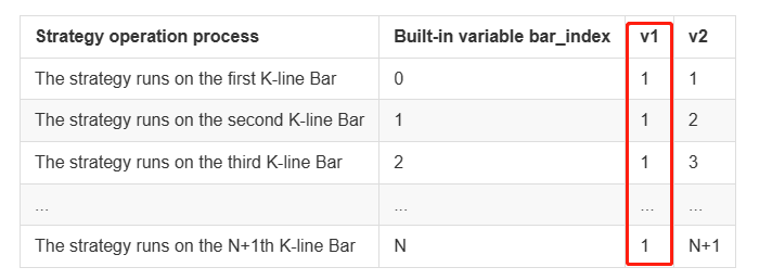
There are many built-in functions like ta.cum that can process data on time series directly. For example, ta.cum is the accumulation of the values corresponding to the variables passed in on each K-line Bar, and next we use a chart to make it easier to understand.

|Strategy operation process|Built-in variable bar_index|v1|v2|
| - | - | - | - |
|The strategy runs on the first K-line Bar|0|1|1|
|The strategy runs on the second K-line Bar|1|1|2|
|The strategy runs on the third K-line Bar|2|1|3|
|…|…|…|…|
|The strategy runs on the N+1th K-line Bar|N|1|N+1|

It can be seen that v1, v2 and even bar_index are all time series structures, and there is corresponding data on each bar. Whether this test code uses the "Bar model" or the "Tick model", the only difference is whether the real-time Bar is displayed on the chart. For quick backtest, we use the "Tick model" to test.

Because the variable v1 is 1 on each Bar, when the ta.cum(v1) function is executed on the first K-line Bar, there is only the first Bar, so the calculation result is 1, assign to variable v2.
When ta.cum(v1) is executed on the second K-line Bar, there are already 2 K-line Bars (the built-in variable bar_index corresponding to the first one is 0, and the second one corresponding to the built-in variable bar_index is 1). The variable bar_index is 1), so the calculation result is 2, which is assigned to the variable v2, and so on. In fact, it can be observed that v2 is the number of K-line Bars in the chart, since the index of the K-line bar_index is incremented from 0, then bar_index + 1 is actually the quantity of K-line Bars. On the chart, we can also see that the lines v2 and bar_index do coincide.

Similarly, I can also use the ta.cum built-in function to calculate the sum of the closing prices of all Bars on the current chart, then just write: ta.cum(close), When the strategy runs to the real-time Bar on the far right, the result calculated by ta.cum(close) is the sum of the closing prices of all Bars on the chart (when it does not run to the far right, it is only accumulated to the current Bar).

Variables on time series can also be operated by using operators, such as code: ta.sma(high - low, 14), put the built-in variable high (the highest price of the K-line Bar) subtract low (the lowest price of K-line Bar), and finally use the ta.sma function to calculate the average value.

Function call results also leave traces of values in the time series

  v1 = ta.highest(high, 10)[1]
  v2 = ta.highest(high[1], 10)
  plot(v1, title="v1", overlay=true)
  plot(v2, title="v2", overlay=true)

The test code is tested during backtesting, and it can be observed that the values of v1 and v2 are the same, and the lines drawn on the chart are also completely coincident. The result calculated by the function call will leave traces of the value in the time series, such as the ta.highest(high, 10) in the code ta.highest(high, 10)[1]. The result calculated by the function call can also use [1] to refer to its historical value. Based on the ta.highest(high, 10) corresponding to the previous bar of the current Bar, the calculation result is ta.highest(high[1], 10). So ta.highest(high[1], 10) and ta.highest(high, 10)[1] are exactly equivalent.

Use another drawing function to output information verification:

  a = ta.highest(close, 10)[1]
  b = ta.highest(close[1], 10)
  plotchar(true, title="a", char=str.tostring(a), location=location.abovebar, color=color.red, overlay=true)
  plotchar(true, title="b", char=str.tostring(b), location=location.belowbar, color=color.green, overlay=true)

We can see that the values of variable a and variable b in the time series are displayed above and below the corresponding Bar. We can keep this drawing code during the learning process, because we may often need to output information on the chart for observation during backtesting.

Script structure

General structure

At the beginning of the tutorial, we have summarized some Pine language differences between FMZ and Trading View. When writing Pine code on FMZ, you can omit the version number, indicator(), strategy(), and library() is currently not supported. Of course, in order to be compatible with earlier versions of Pine scripts, strategies such as: //@version=5, indicator(), strategy() can also be written. Some strategy settings can also be set in the strategy() function.

<version>
<declaration_statement>
<code>

The <version> version control information can be omitted.

Comments

The Pine language uses // as a single-line comment, since the Pine language does not have a multi-line comment. FMZ extends the comment character /**/ for multi-line comments.

Code

Lines in a script that are not comments or compiler directives are statements, which implement the script's algorithm. A statement can be one of these.

Variable declaration
Reassignment of variables
Function declaration
Built-in function calls, user-defined function calls
if, for, while or switch structure

Statements can be arranged in various ways

Some statements can be expressed on one line, such as most variable declarations, lines containing only one function call, or single-line function declarations. Others, like structs, always require multiple lines, because they require a local block.
Statements in the global scope of a script (i.e. parts that are not part of a local block) cannot begin with a space or `tab (tab key). Their first character must also be the first character of the line. Lines that start at the first position of a line are a definition part of the script's global scope.
A struct or multi-line function declaration always requires a local block. A local block must be indented by one tab or four spaces (otherwise, it will be parsed as the concatenated code of the previous line, that is, judged to be the continuous content of the previous line of code), and each local block defines a different local scope.
Multiple single-line statements can be concatenated on a single line by using commas (,) as delimiters.
A line can contain comments or has comments only.
Lines can also be wrapped (continued on multiple lines).

For example, it includes three local blocks, one in the custom function declaration, and two in the variable declaration using the if structure, as follows:

indicator("", "", true)             // declaration statement (global scope), can be omitted

barIsUp() =>                        // function declaration (global scope)
    close > open                    // local block (local scope)

plotColor = if barIsUp()            // variable declaration (global scope)
    color.green                     // local block (local scope)
else
    color.red                       // local block (local scope)

runtime.log("color", color = plotColor)  // Call a built-in function to output the log (global scope)

Line break code

Long lines can be split over multiple lines, or "wrapped". A wrapped line must be indented by any amount of whitespace, as long as it is not a multiple of 4 (these boundaries are used to indent local blocks).

a = open + high + low + close

It can be wrapped as (note that the number of spaces indented per line cannot be a multiple of 4):

a = open +
      high +
          low +
             close

A long plot() call can be wrapped as.

close1 = request.security(syminfo.tickerid, "D", close)      // syminfo.tickerid daily level closing price data series for the current trading pair
close2 = request.security(syminfo.tickerid, "240", close)    // syminfo.tickerid 240-minute level closing price data series for the current trading pair
plot(ta.correlation(close, open, 100),                       // line-long plot() calls can be wrapped
   color = color.new(color.purple, 40),
   style = plot.style_area,
   trackprice = true)

Statements in user-defined function declarations can also be wrapped. However, since a local block must begin with an indent in grammar (4 spaces or 1 tab), when splitting it onto the next line, the continuation of a statement must begin with more than one indent (not equal to 4 multiples of spaces). For example:

test(c, o) =>
    ret = c > o ?
       (c > o+5000 ? 
          1 :
              0):
       (c < o-5000 ? 
          -1 : 
              0)


a = test(close, open)
plot(a, title="a")

Markers and Operators

Markers

Before recognizing variables, we must understand the concept of "markers" first. In layman's terms, "marker" is used as the name of function and variable (used to name variables and functions). Functions will be seen in our later tutorials, let's learn about "markers" first.

1. Markers must begin with an uppercase (A-Z) or lowercase (a-z) letter or an underscore (_) as the first character of the marker.
2. The next character after the first character of a marker can be a letter, underscore, or a number.
3. The naming of markers is case-sensitive.

Such as the following named markers:

fmzVar
_fmzVar
fmz666Var
funcName
MAX_LEN
max_len
maxLen
3barsDown  // Wrong naming! It used a numeric character as the leading character of the marker

Like most programming languages, Pine language has writing suggestions. When naming identifiers, it is generally recommended to:

1. All uppercase letters are used to name constants.
2. Use the lower camel case for other marker names.

// name variables, constants
GREEN_COLOR = #4CAF50
MAX_LOOKBACK = 100
int fastLength = 7

// name functions
zeroOne(boolValue) => boolValue ? 1 : 0

Operators

Operators are some operator symbols used in programming languages to construct expressions, and expressions are computational rules designed for certain computational purposes when we write strategies. Operators in the Pine language are classified by function as:

Assignment operator, arithmetic operator, comparison operator, logical operator, ? : ternary operator, [] historical reference operator.

Taking the arithmetic operator * as an example, it is different from the type problem caused by the return result of the Pine language operator on the Trading View. There is the following test code:

//@version=5
indicator("")
lenInput = input.int(14, "Length")
factor = year > 2020 ? 3 : 1
adjustedLength = lenInput * factor
ma = ta.ema(close, adjustedLength)  // Compilation error!
plot(ma)

When executing this script on Trading View, it will compile and report an error. The reason is that after multiplying adjustedLength = lenInput * factor, the result is series int type (series), but the second parameter of the function ta.ema does not support this type. But there are no such strict restrictions on FMZ, the above code can run normally.

Let's take a look at the use of various operators together.

Assignment Operators

There are 2 types of assignment operators: =, :=, which we have seen in several examples in the beginning part of the tutorial.

The = operator is used to assign a value to a variable when it is initialized or declared. Variables that are initialized, declared and assigned with = will start with that value on each subsequent Bar. These are valid variable declarations:

a = close           // Use built-in variables to assign values to a
b = 10000           // Use numerical assignment
c = "test"          // Use string assignment
d = color.green     // Use color value assignment
plot(a, title="a")
plot(b, title="b")
plotchar(true, title="c", char=str.tostring(c), color=d, overlay=true)

Note that the assignment statement a = close, the variable a on each Bar is the current closing price (close) of the Bar. Other variables b, c, d are unchanged and can be tested in the backtest system on FMZ, and the results can be seen on the chart.

:= is used to reassign values to existing variables. It can be simply understood that the := operator is used to modify the values of variables that have been declared and initialized.
If we use the := operator to assign a value to an uninitialized or declared variable, an error will be raised, for example:

a := 0

Therefore, the := assignment operator is generally used to reassign existing variables, for example:

a = close > open 
b = 0 
if a
    b := b + 1

plot(b)

Judging if close > open (that is, the current BAR is a positive line), the a variable is a true value (true). The code in the local block of the if statement b := b + 1 is executed, and the assignment operator := is used to reassign to b, and 1 is added. Then we use the plot function to draw the value of variable b on each BAR of the time series on the chart, and connect them into a line.

Do we think that when a positive line BAR appears, b will continue to accumulate by 1? Of course not, here we declare and initialize the variable b to 0 without using any keyword designation. This sentence b=0 is executed on each BAR, so we can see that the result of this code is to reset the b variable to 0 every time, if the variable a is true, that is, in line with close > open, then b will be incremented by 1 when the code is executed in this round, and b is 1 when the plot function draws, but b is reassigned to 0 when the code is executed in the next round. This is also the place where Pine language beginners are easy to step on.

When it comes to assignment operators, we must expand on two keywords: var, varip

var In fact, we have seen and used this keyword in previous tutorials, but we did not discuss it in details at that time. Let's look at the description of this keyword first:

var is a keyword used for allocating and one-time initialization of variables. In general, variable assignment grammar that does not contain the keyword var causes the variable's value to be overwritten every time the data is updated. In contrast, when variables are assigned by using the keyword var, they can "keep state" despite data updates.

We still use this example, but we use the var keyword when assigning a value to b here.

  a = close > open 
  var b = 0 
  if a
      b := b + 1

  plot(b)

The var keyword allows the variable b to perform the initial assignment only, and then it will not reset b to 0 every time the strategy logic is executed, so it can be observed from the line drawn at runtime that b is the number of positive line BARs that have appeared when the current K line BAR was backtested.

Variables declared by var can be written not only in the global scope, but also in code blocks, such as this example:

  strategy(overlay=true)
  var a = close
  var b = 0.0
  var c = 0.0
  var green_bars_count = 0
  if close > open
      var x = close
      b := x
      green_bars_count := green_bars_count + 1
      if green_bars_count >= 10
          var y = close
          c := y
  plot(a, title = "a")
  plot(b, title = "b")
  plot(c, title = "c")

The variable 'a' holds the closing price of the first bar in the series.
The variable 'b' holds the closing price of the first 'green' price bar in the series.
The variable 'c' holds the closing price of the tenth 'green' bar in the series.

varip We see the keyword varip for the first time, we can look at the description of this keyword:

varip (var intrabar persist) is a keyword for assigning and one-time initialization of variables. It is similar to the var keyword, but variables declared with varip retain their values when real-time K-line updates.

Is it difficult to understand? It doesn't matter, we explain it through an example, it is easy to understand.

  strategy(overlay=true)

  // test var varip
  var i = 0
  varip ii = 0  

  // Print the i and ii changed in each round of the strategy logic on the chart
  plotchar(true, title="ii", char=str.tostring(ii), location=location.abovebar, color=color.red)
  plotchar(true, title="i", char=str.tostring(i), location=location.belowbar, color=color.green)  

  // Increment i and ii by 1 for each round of logic execution
  i := i + 1
  ii := ii + 1

This test code has different performances on "Bar Model" and "Tick Model":

Bar Model:
Do you remember that the strategy execution we explained earlier is divided into historical BAR stage and real-time BAR stage? In the Bar Model, the historical K-line stage, the variables i, ii declared in var, varip perform incremental operations at each round of execution of the strategy code. Therefore, it can be seen that the numbers displayed on the K-line BAR of the backtest result are incremented by 1 one by one. When the historical K-line stage ends, the real-time K-line stage begins. The variables declared by var and vrip start to change differently. Because it is Bar Model, the strategy code will be executed once for each price change in a K-line BAR, i := i + 1 and ii := ii + 1 will be executed once. The difference is that ii is modified every time. Although i is modified every time, the previous value will be restored when the strategy logic is executed in the next round (remember the rollback mechanism we explained in the previous "Model Execution" chapter?), and the value of i will not be updated until the current K-line BAR is completed. value (that is, the previous value will not be restored when the strategy logic is executed in the next round). So it can be seen that the variable i is still increased by 1 for each BAR. But variable ii is accumulated several times for each BAR.

Tick Model:
Since the Tick Model executes the strategy logic only once per K-line BAR. So in the closing price model, the variables declared by var and varip behave exactly the same in the above example incrementing by 1 for each K-line BAR during the historical K-line stage and the real-time K-line stage.

Arithmetic Operators

|Operators|Description|
|-|-|
|+|Addition|
|-|Subtraction|
|*|Multiplication|
|/|Division|
|%|Modulo|

The + and - operators can be used as binary operators or as unary operators. Other arithmetic operators can only be used as binary operators and it will report an error if it was used as unary operators.

Both sides of the arithmetic operator are numeric type, the result is a numeric type, integer or floating point depending on the result of the operation.
If one of the operands is a string and the operator is +, the result of the calculation is a string, the value will be converted to the string form, and then the strings are stitched together. If it is other arithmetic operator, it will try to convert the string to a value and then carry on the operation.
If one of the operands is na, the result of the calculation is the null value--na, and it will show NaN when printed on FMZ.

a = 1 + 1 
b = 1 + 1.1
c = 1 + "1.1"
d = "1" + "1.1"
e = 1 + na 

runtime.log("a:", a, ", b:", b, ", c:", c, ", d:", d, ", e:", e)   
// a: 2 , b: 2.1 , c: 11.1 , d: 11.1 , e: NaN

The Pine language on FMZ is a little different from the Pine language on Trading View, the Pine language on FMZ is not very strict about variable types. For example:

a = 1 * "1.1"
b = "1" / "1.1"
c = 5 % "A" 

plot(a)
plot(b)
plot(c)

It works on FMZ, but it reports a type error on the Trading View. If both operands of the arithmetic operator are strings, the system converts the strings to numeric values and then calculates them. If a non-numeric string cannot be computed, the result of the system operation is a null value--na.

Comparison Operators

The comparison operators are all binary operators.

|Operators|Description|
|-|-|
|<|<| |>|>|
|<=|<=|

>=	>=
!=	!=

Test example:

a = 1 > 2 
b = 1 < 2 
c = "1" <= 2 
d = "1" >= 2 
e = 1 == 1 
f = 2 != 1 
g = open > close 
h = na > 1 
i = 1 > na

runtime.log("a:", a, ", b:", b, ", c:", c, ", d:", d, ", e:", e, ", f:", f, ", g:", g, ", h:", h, ", i:", i)   
// a: false , b: true , c: true , d: false , e: true , f: true , g: false , h: false , i: false

As we can see, the comparison operator is very simple to use, but this is also the operator we use the most when writing strategies. Both numeric values and built-in variables can be compared, such as close, open, etc.
As with the operator, there is a difference about Pine language between FMZ and Trading View. FMZ does not have particularly strict requirements for types, so such statements d = "1" >= 2 will not report an error on FMZ, and it will be executed by converting the string to a value first and then comparing the operation. On Trading View, it will report an error.

Logical Operators

|Operators|Code Symbols|Description|
|-|-|-|
|not|not|Unary operator, not operations|
|and|and|Binary operators, and operations|
|or|or|Binary operators, or operations|

When it comes to logical operators, then we must talk about truth tables. The same as we learned in high school, here we just test and learn in our backtesting system:.

a = 1 == 1  // An expression formed by using comparison operators, the result is a Boolean value
b = 1 != 1
c = not b   // Logical not operators
d = not a   // Logical not operators

runtime.log("test the logical operator：and", "#FF0000")
runtime.log("a:", a, ", c:", c, ", a and c:", a and c)
runtime.log("a:", a, ", b:", b, ", a and b:", a and b)
runtime.log("b:", b, ", c:", c, ", b and c:", b and c)
runtime.log("d:", d, ", b:", b, ", d and b:", d and b)

runtime.log("test the logical operator：or", "#FF0000")
runtime.log("a:", a, ", c:", c, ", a or c:", a or c)
runtime.log("a:", a, ", b:", b, ", a or b:", a or b)
runtime.log("b:", b, ", c:", c, ", b or c:", b or c)
runtime.log("d:", d, ", b:", b, ", d or b:", d or b)

runtime.error("stop")

In order not to overprint the message, we throw an error with the runtime.error("stop") and make it stop after printing once. After that, we can observe the output information, and we can find that the printed content is actually the same as the truth table.

Ternary Operator

Ternary expressions using the ternary operator ? : combined with operands condition ? valueWhenConditionIsTrue : valueWhenConditionIsFalse We have also used them in the previous lessons. The so-called ternary expression, ternary operator means that there are three operands in it.

in the condition ? valueWhenConditionIsTrue : valueWhenConditionIsFalse, condition is the judgment condition. If it is true, the value of the expression is: valueWhenConditionIsTrue. If ``conditionis false, then the value of the expression isvalueWhenConditionIsFalse```.

Example of a convenient demonstration, although of little practical use:

a = close > open
b = a ? "positive line" : "negative line"
c = not a ? "negative line" : "positive line"
plotchar(a, location=location.abovebar, color=color.red, char=b, overlay=true)
plotchar(not a, location=location.belowbar, color=color.green, char=c, overlay=true)

What to do if we encounter a doji? It doesn't matter! Ternary expressions can also be nested, as we did in the previous tutorial.

a = close > open
b = a ? math.abs(close-open) > 30 ? "positive line" : "doji" : math.abs(close-open) > 30 ? "negative line" : "doji"
c = not a ? math.abs(close-open) > 30 ? "negative line" : "doji" : math.abs(close-open) > 30 ? "positive line" : "doji"
plotchar(a, location=location.abovebar, color=color.red, char=b, overlay=true)
plotchar(not a, location=location.belowbar, color=color.green, char=c, overlay=true)

In fact, it is equivalent to replacing valueWhenConditionIsTrue and valueWhenConditionIsFalse in condition ? valueWhenConditionIsTrue : valueWhenConditionIsFalse with another ternary expression.

Historical Operator

Use the historical operator [] to refer to historical values on a time series. These historical values are the values of the variable on the K-line bar before the current K-line bar when the script was running. The [] operator is used after variables, expressions, and function calls. []The value in square brackets is the offset of the historical data we want to reference from the current K-line BAR. For example, if I want to quote the closing price of the last K-line BAR, we write it as: close[1].

We've seen something like this in the previous lessons:

high[10]
ta.sma(close, 10)[1]
ta.highest(high, 10)[20]
close > nz(close[1], open)

The [] operator can only be used once on the same value, so it is wrong to write it like this, and an error will be reported:

a = close[1][2]   // error

Here, someone may say that the operator [] is used for series structure, it seems that series structure (series) is similar to array!
Let's use an example to illustrate the difference between series and arrays in the Pine language.

strategy("test", overlay=true)

a = close
b = close[1]
c = b[1]

plot(a, title="a")
plot(b, title="b")
plot(c, title="c")

a = close[1][2]will report an error, but：

b = close[1]
c = b[1]

But if written separately, it will not report an error. If we understand it according to the usual array, after the assignment of b = close [1], b should be a value, but c = b[1], b can still be used to refer to the historical value again by using the history operator. It can be seen that the concept of series in the Pine language is not as simple as an array. It can be understood as the historical value on the last bar of close (assigned to b), b is also a time series structure (time series), and its historical value can continue to be referenced. So we see that in the drawn three lines a, b, and c, line b is one BAR slower than line a, and line c is one BAR slower than line b. The line-c is 2 BAR slower than the line-a.

We can pull the chart to the far left and observe that on the first K-line, the values of b and c are both null (na). That's because when the script is executed on the first K-line BAR, it does not exist when referring to the historical value of one or two periods forward, which does not exist. Therefore, we need to always pay attention to whether the null value will be referenced when referring to the historical data when writing the strategy. If the null value is used carelessly, it will cause a series of calculation differences, and may even affect the real-time BAR. Usually we will use built-in functions na, nz to judge in the code (in fact, we have also touched nz, `na in our previous vedios, do you remember which one it is?) deal with the case of null values, for example:

close > nz(close[1], open)    // When referencing the history value of the previous BAR of the close built-in variable, if it does not exist, the open built-in variable is used

This is a handling of possible references to null values (na).

Operator Priority

We have learned a lot of Pine language operators. These operators form expressions through various combinations with operands. So what is the priority of these operations when evaluating in expressions? For example, when we were in school, we learned the four operations, multiplication and division is the first to calculate, and then calculate addition and subtraction. The same is true of expressions in the Pine language.

|Priority|Operators|
|-|-|
|9|[]|
|8|+ 、-andnot in the unary operator|
|7|*、/、%|
|6|+、- in the binary operator|
|5|>、<、>=、<=|
|4|==、!=|
|3|and|
|2|or|
|1|?:|

The part of the expression with higher precedence is evaluated first, and if the precedence is the same, it is evaluated from left to right. If you want to force a part to be evaluated first, you can use () to wrap the expression to force the part to be evaluated first.

Variables

Variable Declaration

We have already studied the concept of "marker", which is used as the name of a variable, that is, a variable is a marker that holds a value. So how do we declare a variable? What are the rules for declaring variables?

Declaration Mode:
The first thing to write when declaring a variable is the "declaration mode". There are three declaration modes for variables, namely:

Use the keyword var.
Use the keyword varip.
Write nothing. The var and varip keywords have actually been studied in our previous chapter on Assignment Operators'', so we won't repeat them here. If the declaration mode of a variable is written without anything, for example, the statement:i = 1```, as we have actually talked about before, such a variable declared and assigned is executed on every K-line BAR.

Type
The Pine language on FMZ is not strict with type requirements and it can generally be omitted. However, in order to be compatible with the scripting strategy on Trading View, variables can also be declared with types. For example:

  int i = 0 
  float f = 1.1

The type on the Trading View is more stringent, and an error will be reported if the following code is used on the Trading View:

  baseLine0 = na          // compile time error!

Marker
Markers are variable names. The naming of markers has been mentioned in the previous video, so you can go back and watch the previous video: https://www.fmz.com/bbs-topic/9390#%E6%A0%87%E8%AF%86%E7%AC%A6

To summarize, declaring a variable can be written as:

// [<declaration_mode>] [<type>] <marker> = value 
   declaration mode             type     marker      = value

The assignment operator is used here: = assigns a value to a variable when it is declared. When assigning, the value can be a string, number, expression, function call, if, for, while, or switch and other structures (These structural keywords and statement usage will be explained in detail in the follow-up courses. In fact, we have learned simple if statement assignments in the previous courses, you can review them).

Here we focus on the input function, which is a function that we will use frequently when designing and writing strategies. It is also a very critical function when designing strategies.

input function:

inputfunction, parameters: defval、title、tooltip、inline、group

The input function on FMZ is somewhat different from that on Trading View, but this function is used as the assignment input of strategy parameters. Let's use an example to illustrate the use of the input function on FMZ in details:

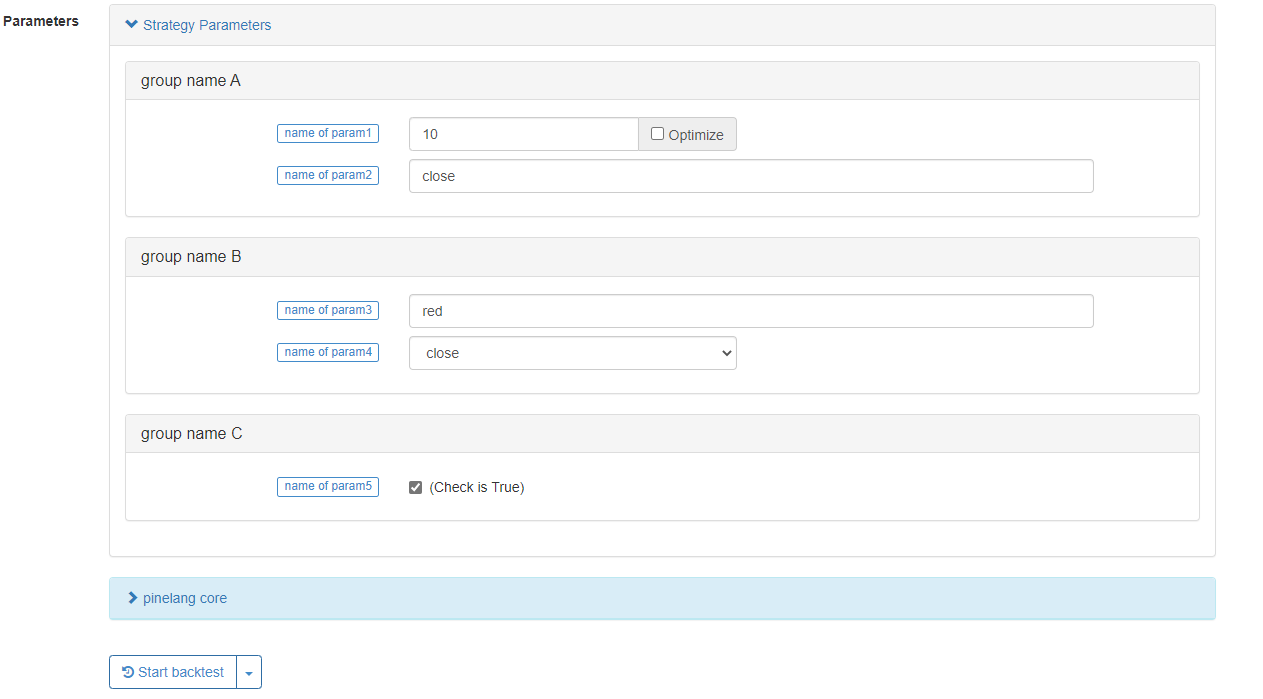
param1 = input(10, title="name of param1", tooltip="description for param1", group="group name A")
param2 = input("close", title="name of param2", tooltip="description for param2", group="group name A")
param3 = input(color.red, title="name of param3", tooltip="description for param3", group="group name B")
param4 = input(close, title="name of param4", tooltip="description for param4", group="group name B")
param5 = input(true, title="name of param5", tooltip="description for param5", group="group name C")

ma = ta.ema(param4, param1)
plot(ma, title=param2, color=param3, overlay=param5)

The input function is often used to assign values to variables when declaring them. input function on FMZ draws controls for setting strategy parameters automatically in the FMZ strategy interface. The controls supported on FMZ currently include numeric input boxes, text input boxes, drop-down boxes, and Boolean checkboxes. And you can set the strategy parameter grouping, set the parameter prompt text message and other functions.

We introduce several main parameters of the input function.

defval : As the default value of the strategy parameter option set by the input function, it supports built-in variables, values, and strings of the Pine language.
title : The parameter name of the strategy displayed on the strategy interface of the real bot/backtest.
tooltip : The prompt information of the strategy parameter, when the mouse hovers over the strategy parameter, the text information of the parameter setting will be displayed.
group : The name of the strategy parameter group, which can be used to strategy parameters.

In addition to individual variable declaration and assignment, there is also a way of declaring a group of variables and assigning them in the Pine language:

[Variable A, Variable B, Variable C] = function or structure such as ```if```, ```for```, ```while``` or ```switch```

The most common is that when we use the ta.macd function to calculate the MACD indicator, since the MACD indicator is a multi-line indicator, three sets of data are calculated. So it can be written as:

[dif,dea,column] = ta.macd(close, 12, 26, 9)

plot(dif, title="dif")
plot(dea, title="dea")
plot(column, title="column", style=plot.style_histogram)

We can draw the MACD chart using the above code easily. Not only the built-in functions can return to multiple variables, but also the written custom functions can return to multiple data.

twoEMA(data, fastPeriod, slowPeriod) =>
    fast = ta.ema(data, fastPeriod)
    slow = ta.ema(data, slowPeriod)

[fast, slow]

[ema10, ema20] = twoEMA(close, 10, 20) plot(ema10, title="ema10", overlay=true) plot(ema20, title="ema20", overlay=true)

The writing method of using if and other structures as multiple variable assignments is also similar to the above custom function, and you can try it if you are interested.

[ema10, ema20] = if true
    fast = ta.ema(close, 10)
    slow = ta.ema(close, 20)

[fast, slow]

plot(ema10, title="ema10", color=color.fuchsia, overlay=true) plot(ema20, title="ema20", color=color.aqua, overlay=true)

Condition Structure

Some functions cannot be written in the local code block of the conditional branch, mainly are the following functions:

barcolor(), fill(), hline(), indicator(), plot(), plotcandle(), plotchar(), plotshape()

Trading View will report errors, FMZ is not as restrictive, but it is recommended to follow the specifications of Trading View. For example, although this does not report an error on FMZ, it is not recommended.

strategy("test", overlay=true)
if close > open 
    plot(close, title="close")
else 
    plot(open, title="open")

if statement

Lecture example:

var lineColor = na

n = if bar_index > 10 and bar_index <= 20
    lineColor := color.green
else if bar_index > 20 and bar_index <= 30
    lineColor := color.blue
else if bar_index > 30 and bar_index <= 40
    lineColor := color.orange
else if bar_index > 40
    lineColor := color.black
else 
    lineColor := color.red

plot(close, title="close", color=n, linewidth=5, overlay=true)
plotchar(true, title="bar_index", char=str.tostring(bar_index), location=location.abovebar, color=color.red, overlay=true)

Focus: Expressions used for judgments that return Boolean values. Note the indentation. There can be at most one else branch. If all branch expressions are not true and there is no else branch, return na.

x = if close > open
    close
plot(x, title="x")

switch statement

The switch statement is also a branch-structured statement, which is used to design different paths to be executed according to certain conditions. Generally, the switch statement has the following key knowledge points.

The switch statement, like the if statement, can also return a value.
Unlike switch statements in other languages, when a switch construct is executed, only a local block of its code is executed, so the break statement is unnecessary (ie, there is no need to write keywords such as break).
Each branch of switch can write a native code block, the last line of this native code block is the return value (it can be a tuple of values). Returns na if none of the branched native code blocks were executed.
The expression in the switch structure determines the position can write a string, variable, expression or function call.
switch allows specifying a return value that acts as the default value to be used when there is no other case in the structure to execute.

There are two forms of switch, let's look at the examples one by one to understand their usage.

switch with expressions
example to explain

// input.string: defval, title, options, tooltip
func = input.string("EMA", title="indicator name", tooltip="select the name of the indicator function to be used", options=["EMA", "SMA", "RMA", "WMA"])

// input.int: defval, title, options, tooltip
// param1 = input.int(10, title="period parameter")
fastPeriod = input.int(10, title="fastPeriod parameter", options=[5, 10, 20])
slowPeriod = input.int(20, title="slowPeriod parameter", options=[20, 25, 30])

data = input(close, title="data", tooltip="select the closing price, opening price, highest price...")
fastColor = color.red
slowColor = color.red

[fast, slow] = switch func
    "EMA" =>
        fastLine = ta.ema(data, fastPeriod)
        slowLine = ta.ema(data, slowPeriod)
        fastColor := color.red
        slowColor := color.red
        [fastLine, slowLine]
    "SMA" =>
        fastLine = ta.sma(data, fastPeriod)
        slowLine = ta.sma(data, slowPeriod)
        fastColor := color.green
        slowColor := color.green
        [fastLine, slowLine]
    "RMA" =>
        fastLine = ta.rma(data, fastPeriod)
        slowLine = ta.rma(data, slowPeriod)
        fastColor := color.blue
        slowColor := color.blue
        [fastLine, slowLine]
    =>
        runtime.error("error")
        
plot(fast, title="fast" + fastPeriod, color=fastColor, overlay=true)
plot(slow, title="slow" + slowPeriod, color=slowColor, overlay=true)

We learned the input function before, here we continue to learn two functions similar to input: input.string, input.int functions.
input.string is used to return a string, and the input.int function is used to return an integer value. In the example, there is a new usage of the options parameter. The options parameter can be passed an array of optional values. For example options=["EMA", "SMA", "RMA", "WMA"] and options=[5, 10, 20] in the example (note that one is string type, one is a numeric type). In this way, the controls on the strategy interface do not need to input specific values, but the controls become drop-down boxes to select these options provided in the options parameter.

The value of the variable func is a string, and the variable func is used as the expression of the switch (which can be a variable, function call, expression) to determine which branch in the switch is executed. If the variable func cannot match (ie, equal) the expression on any branch in the switch, the default branch code block will be executed, and the runtime.error("error") function will be executed, causing the strategy to stop.

In our test code above, after the last line of runtime.error in the default branch code block of switch, we did not add code like [na, na] to be compatible with the return value. This problem needs to be considered in the trading view. If If the type is inconsistent, an error will be reported. But on FMZ, since the type is not strictly required, this compatibility code can be omitted. Therefore, there is no need to consider the type compatibility of the return value of if and switch branches on FMZ.

strategy("test", overlay=true)
x = if close > open
    close
else
    "open"
plotchar(true, title="x", char=str.tostring(x), location=location.abovebar, color=color.red)

No error will be reported on FMZ, but an error will be reported on trading view. Because the type returned by the if branch is inconsistent.

switch without expressions

Next, let's look at another way to use switch, that is, without expressions.

up = close > open     // up = close < open 
down = close < open 
var upOfCount = 0 
var downOfCount = 0 

msgColor = switch
    up  => 
        upOfCount += 1 
        color.green 
    down => 
        downOfCount += 1
        color.red

plotchar(up, title="up", char=str.tostring(upOfCount), location=location.abovebar, color=msgColor, overlay=true)
plotchar(down, title="down", char=str.tostring(downOfCount), location=location.belowbar, color=msgColor, overlay=true)

As we can see from the test code example, switch will match the execution of the local code block that is true on the branch condition. In general, the branch conditions following a switch statement must be mutually exclusive. That is to say, up and down in the example cannot be true at the same time. Because switch can only execute the local code block of one branch, if you are interested, you can replace this line in the code: up = close > open // up = close < open to the content in the comment, and backtest to observe the result. You will find that the switch branch can only execute the first branch. In addition, it is necessary to pay attention not to write function calls in the branch of switch as much as possible, the function cannot be called on each BAR may cause some data calculation problems (unless as in the example of "switch with expressions", the execution branch is deterministic and will not be changed while the strategy is running).

Loop Structure

for statement

return value = for count = start count to final count by step length
    statement                                            // Note: There can be break and continue in the statement
    statement                                            // Note: The last statement is the return value

The for statement is very simple to use, the for loop can finally return to a value (or return to multiple values, in the form of [a, b, c]). Like the variable assigned to the "return value" position in the pseudocode above. The for statement is followed by a "count" variable used to control the number of loops, refer to other values, etc. The "count" variable is assigned the "initial count" before the loop starts, then increments according to the "step length" setting, and the loop stops when the "count" variable is greater than the "final count".

The break keyword used in the for loop: the loop stops when the break statement is executed.
The continue keyword used in the for loop: When the continue statement is executed, the loop will ignore the code after continue and execute the next round of the loop directly. The for statement returns to the return value from the last execution of the loop. And it returns null if no code is executed.

Then we use a simple example to demonstrate:

ret = for i = 0 to 10       // We can increase the keyword by to modify the step length, FMZ does not support reverse loops such as i = 10 to 0 for now
    // We can add condition settings, use continue to skip, use break to jump out
    runtime.log("i:", i)
    i                       // If this line is not written, it will return null because there is no variable to return
    
runtime.log("ret:", ret)
runtime.error("stop")

for ... in statement

The for ... in statement has two forms, we will illustrat them in the following pseudocode.

return value = for array element in array 
    statement                        // Note: There can be break and continue in the statement
    statement                        // Note: The last statement is the return value

Return value = for [index variable, array element corresponding to index variable] in array
    statement                        // Note: There can be break and continue in the statement
    statement                        // Note: The last statement is the return value

We can see that the main difference between the two forms is the content that follows the for keyword. One is to use a variable as a variable that refers to the elements of the array. One is to use a structure containing index variables, tuples of array element variables to reference. For other return value rules, the use of break, continue and other rules is consistent with the for loop. We also illustrate the use with a simple example.

testArray = array.from(10, 20, 30, 40, 50, 60, 70, 80, 90, 100)
for ele in testArray            // Modify it to the form of [i, ele]: for [i, ele] in testArray, runtime.log("ele:", ele, ", i:", i)
    runtime.log("ele:", ele)

runtime.error("stop")

When it need to use the index, use for [i, ele] in testArray.

Application of for loops

We can use the built-in functions provided in the Pine language to complete some of the loop logic calculations, either written by using the loop structure directly or processed using the built-in functions. Let's take two examples:

Calculate the mean value

When designing with a loop structure:

length = 5
var a = array.new(length)
array.push(a, close)

if array.size(a) >= length
	array.remove(a, 0)
	
sum = 0 	
for ele in a
    sum += ele 

avg = sum / length
plot(avg, title="avg", overlay=true)

The example uses a for loop to sum and then calculate the mean value.

Calculate the moving average directly by using the built-in function:

plot(ta.sma(close, length), title="ta.sma", overlay=true)

Use the built-in function ta.sma directly to calculate the moving average indicator. Obviously, it is simpler to use the built-in function for calculating the moving average. Comparing on the chart, it can be seen that the calculated results are completely consistent.

We still use the example above to illustrate.

When designing with a loop structure:

length = 5
var a = array.new(length)
array.push(a, close)

if array.size(a) >= length
	array.remove(a, 0)
	
sum = 0 	
for ele in a
    sum += ele 

avg = sum / length
plot(avg, title="avg", overlay=true)
plot(ta.sma(close, length), title="ta.sma", overlay=true)

For calculating the sum of all elements of an array, we can use a loop to process it, or use the built-in function array.sum to calculate.
Calculate the sum directly by using the built-in function:

length = 5
var a = array.new(length)
array.push(a, close)

if array.size(a) >= length
	array.remove(a, 0)
	
plot(array.sum(a) / length, title="avg", overlay=true)
plot(ta.sma(close, length), title="ta.sma", overlay=true)

We can see the calculated data is exactly the same as that displayed on the chart using plot.

So why design loops when we can do all these with built-in functions? The use of loops is mainly based on the application of these 3 points:

For some operations on arrays, calculations.
To review the history, for example, to find out how many past high points are higher than the current BAR high point. Since the high point of the current BAR is only known at the BAR where the script is running, a loop is needed to return and analyze the past BAR in time.
The use of the built-in functions of the Pine language cannot complete the calculation of past BARs.

while statemnet

The while statement keeps the code in the loop section executing until the condition in the while structure is false.

return value = while judgment condition
    statement                    // Note: There can be break and continue in the statement
    statement                    // Note: The last statement is the return value

The other rules of while are similar to those of the for loop. The last line of the local code block of the loop body is the return value, which can return multiple values. Execute the loop when the "loop condition" is true, and stop the loop when the condition is false. The break and continue statements can also be used in the loop body.

We will still use the example of calculating averages for demonstration:

length = 10

sma(data, length) => 
    i = 0 
    sum = 0 
    while i < 10 
        sum += data[i]
        i += 1
        sum / length

plot(sma(close, length), title="sma", overlay=true)
plot(ta.sma(close, length), title="ta.sma", overlay=true)

As you we see that the while loop is also very simple to use, and it is also possible to design some calculation logic that cannot be replaced by the built-in functions, such as calculating factorial:

counter = 5
fact = 1

ret = while counter > 0
    fact := fact * counter
    counter := counter - 1
    fact

plot(ret, title="ret")  // ret = 5 * 4 * 3 * 2 * 1

Arrays

The definition of arrays in the Pine language is similar to that in other programming languages. Pine's arrays are one-dimensional arrays. Usually it's used to store a continuous series of data. The single data stored in the array is called the element of the array, and the types of these elements can be: integer, floating point, string, color value, boolean value. The Pine language on FMZ is not very strict about types, and it can even store strings and numbers in an array at the same time. Since the bottom layer of the array is also a series structure, if the historical operator is used to refer to the array state on the previous BAR. So instead of using the history operator [] to refer to an element in the array, we need to use the functions array.get() and array.set() . The index order of the elements in the array is that the index of the first element of the array is 0, and the index of the next element is incremented by 1.

We illustrate it with a simple code:

var a = array.from(0)
if bar_index == 0 
    runtime.log("current value a on BAR:", a, ", a on the last BAR, i.e. the value of a[1]:", a[1])
else if bar_index == 1 
    array.push(a, bar_index)
    runtime.log("current value a on BAR:", a, ", a on the last BAR, i.e. the value of a[1]:", a[1])
else if bar_index == 2
    array.push(a, bar_index)
    runtime.log("current value a on BAR:", a, ", a on the last BAR, i.e. the value of a[1]:", a[1], ", a on the last second BAR, i.e. the value of a[2]:", a[2])
else if bar_index == 3 
    array.push(a, bar_index)
    runtime.log("current value a on BAR:", a, ", a on the last BAR, i.e. the value of a[1]:", a[1], ", a on the last second BAR, i.e. the value of a[2]:", a[2], ", a on the last third BAR, i.e. the value of a[3]:", a[3])
else if bar_index == 4 
    // Obtain elements by index using array.get, modify elements by index using array.set
    runtime.log("Before array modification:", array.get(a, 0), array.get(a, 1), array.get(a, 2), array.get(a, 3))
    array.set(a, 1, 999)
    runtime.log("After array modification:", array.get(a, 0), array.get(a, 1), array.get(a, 2), array.get(a, 3))

Arrays Declaration

Arrays can be assigned arrays by using array<int> a, float[] b or by declaring only one variable, for example:

array<int> a = array.new(3, bar_index)
float[] b = array.new(3, close)
c = array.from("hello", "fmz", "!")
runtime.log("a:", a)
runtime.log("b:", b)
runtime.log("c:", c)
runtime.error("stop")

Array variables are initialized by using the array.new and array.from functions. There are also many types-related functions similar to array.new in the Pine language: array.new_int(), array.new_bool(), array.new_color() , array.new_string(), etc.

The var keyword also works with the array declaration mode. Arrays declared with the var keyword are initialized only on the first BAR. Let's observe with an example:

var a = array.from(0)
b = array.from(0)

if bar_index == 1
    array.push(a, bar_index)
    array.push(b, bar_index)
else if bar_index == 2 
    array.push(a, bar_index)
    array.push(b, bar_index)
else if barstate.islast
    runtime.log("a:", a)
    runtime.log("b:", b)
    runtime.error("stop")

It can be seen that the changes of the array a have been continuously determined and have not been reset. The array b is initialized on each BAR. Finally, when barstate.islast is true, there is still only one element--the value 0.

Read and write elements in an array

Use array.get to get the element at the specified index position in the array, and use array.set to modify the element at the specified index position in the array.

The first parameter of array.get is the array to be processed, and the second parameter is the specified index.
The first parameter to array.set is the array to be processed, the second argument is the specified index, and the third argument is the element to be written.

We use the following simple example to illustrate:

lookbackInput = input.int(100)
FILL_COLOR = color.green

var fillColors = array.new(5)
if barstate.isfirst
    array.set(fillColors, 0, color.new(FILL_COLOR, 70))
    array.set(fillColors, 1, color.new(FILL_COLOR, 75))
    array.set(fillColors, 2, color.new(FILL_COLOR, 80))
    array.set(fillColors, 3, color.new(FILL_COLOR, 85))
    array.set(fillColors, 4, color.new(FILL_COLOR, 90))

lastHiBar = - ta.highestbars(high, lookbackInput)
fillNo = math.min(lastHiBar / (lookbackInput / 5), 4)

bgcolor(array.get(fillColors, int(fillNo)), overlay=true)
plot(lastHiBar, title="lastHiBar")
plot(fillNo, title="fillNo")

The example initializes the base color green, declares and initializes an array to hold the colors, and then assigns different transparency to the color values (by using the color.new function). The color level is calculated by calculating the distance of the current BAR from the maximum value of high in 100 lookback periods. The closer the distance to the maximum value of HIGH in the last 100 lookback cycles, the higher the rank and the darker (less transparent) the corresponding color value. Many similar strategies use this way to represent the current price level within N lookback periods.

Iterate through array elements

How to iterate through an array, we use the for/for in/while statements that we have learned before can be implemented.

a = array.from(1, 2, 3, 4, 5, 6)

for i = 0 to (array.size(a) == 0 ? na : array.size(a) - 1)
    array.set(a, i, i)
    
runtime.log(a)
runtime.error("stop")

a = array.from(1, 2, 3, 4, 5, 6)

i = 0
while i < array.size(a)
    array.set(a, i, i)
    i += 1

runtime.log(a)
runtime.error("stop")

a = array.from(1, 2, 3, 4, 5, 6)

for [i, ele] in a 
    array.set(a, i, i)

runtime.log(a)
runtime.error("stop")

These three traversal methods have the same result.

Arrays can be declared in the global scope of a script, or in the local scope of a function or if branch

Historical data references

For the use of elements in arrays, the following ways are equivalent. We can see by the following example that two sets of lines are drawn on the chart, two in each set, and the two lines in each set have exactly the same value.

a = array.new_float(1)
array.set(a, 0, close)
closeA1 = array.get(a, 0)[1]
closeB1 = close[1]
plot(closeA1, "closeA1", color.red, 6)
plot(closeB1, "closeB1", color.black, 2)

ma1 = ta.sma(array.get(a, 0), 20)
ma2 = ta.sma(close, 20)
plot(ma1, "ma1", color.aqua, 6)
plot(ma2, "ma2", color.black, 2)

Functions for adding and deleting arrays

Functions related to the adding operation of arrays:

array.unshift(), array.insert(), array.push().

Functions related to the deleting operation of arrays:

array.remove(), array.shift(), array.pop(), array.clear().

We use the following example to test these array adding and deleting operation functions.

a = array.from("A", "B", "C")
ret = array.unshift(a, "X")
runtime.log("array a:", a, ", ret:", ret)

ret := array.insert(a, 1, "Y")
runtime.log("array a:", a, ", ret:", ret)

ret := array.push(a, "D")
runtime.log("array a:", a, ", ret:", ret)

ret := array.remove(a, 2)
runtime.log("array a:", a, ", ret:", ret)

ret := array.shift(a)
runtime.log("array a:", a, ", ret:", ret)

ret := array.pop(a)
runtime.log("array a:", a, ", ret:", ret)

ret := array.clear(a)
runtime.log("array a:", a, ", ret:", ret)

runtime.error("stop")

Application of additions, deletions: arrays as queues

We can construct a "queue" data structure by using arrays and some functions of adding and deleting arrays. Queues can be used to calculate the moving average of tick prices. Someone may ask, "Why should we construct a queue structure? Didn't we use arrays to calculate the average before?"

A queue is a structure that is often used in the field of programming, the characteristics of a queue are:

The element that enters the queue first, leaves the queue first.

This ensures that the data in the queue is the latest data, and that the length of the queue will not expand indefinitely (unlimited expansion code can only be written at noon, because "morning" and "evening" will cause problems).

In the following example, we use a queue structure to record the price of each tick, calculate the mobile average price at the tick level, and then compare it with the moving average at the 1-minute K-line level.

strategy("test", overlay=true)

varip a = array.new_float(0)
var length = 10

if not barstate.ishistory
    array.push(a, close)

    if array.size(a) > length
        array.shift(a)

sum = 0.0
for [index, ele] in a 
    sum += ele

avgPrice = array.size(a) == length ? sum / length : na

plot(avgPrice, title="avgPrice")
plot(ta.sma(close, length), title="ta.sma")

Note that when declaring array a, we specify the declaration mode and use the keyword variant. In this way, each price change will be recorded in array a.

Array calculation and operation functions commonly used

Calculate correlation functions:

array.avg() calculates the average value of all elements in an array, array.min() calculates the smallest element in an array, array.max()calculates the smallest element in an array, array.stdev() calculates the standard deviation of all elements in an array, array.sum() calculates the standard deviation of all elements in an array.

Operation-related functions:
array.concat() to merge or concatenate two arrays.
array.copy() to copy the array.
array.join to concatenates all the elements of an array into a string.
array.sort() to sort by ascending or descending order.
array.reverse() to reverse the array.
array.slice() to slice the array.
array.includes() to judge the element.
array.indexof() to return to the index of the first occurrence of the value passed in as a parameter. If the value is not found, -1 is returned.
array.lastindexof() to find the last occurrence of the value.

Test examples of array calculation-related functions:

a = array.from(3, 2, 1, 4, 5, 6, 7, 8, 9)

runtime.log("avg:", array.avg(a))
runtime.log("min:", array.min(a))
runtime.log("max:", array.max(a))
runtime.log("stdev:", array.stdev(a))
runtime.log("sum:", array.sum(a))
runtime.error("stop")

These are commonly used array calculation functions.

Examples of operation-related functions:

a = array.from(1, 2, 3, 4, 5, 6)
b = array.from(11, 2, 13, 4, 15, 6)

runtime.log("array a: ", a, ", array b: ", b)
runtime.log("array a, array b is concatenated with:", array.concat(a, b))
c = array.copy(b)

runtime.log("Copy an array b and assign it to the variable c, variable c:", c)

runtime.log("use array.join to process the array c, add the symbol + to the middle of each element, concatenating all elements results in a string:", array.join(c, "+"))
runtime.log("Sort the array b, in order from smallest to largest, using the parameter order.ascending:", array.sort(b, order.ascending))     // array.sort function modifies the original array
runtime.log("Sort the array b, in order from largest to smallest, using the parameter order.descending:", array.sort(b, order.descending))   // array.sort function modifies the original array

runtime.log("array a:", a, ", array b:", b)
array.reverse(a)   // This function modifies the original array
runtime.log("reverse the order of all elements in the array a, after reversing, the array a is:", a)    

runtime.log("Intercept array a, index 0~index 3, and follow the rule of left-closed and right-open interval:", array.slice(a, 0, 3))
runtime.log("Search for element 11 in array b:", array.includes(b, 11))
runtime.log("Search for element 100 in array a:", array.includes(a, 100))
runtime.log("Connect array a and array b, and search the index position of the first occurrence of element 2:", array.indexof(array.concat(a, b), 2), " , observe array.concat(a, b):", array.concat(a, b))
runtime.log("Connect array a and array b, and search the index position of the last occurrence of element 6:", array.lastindexof(array.concat(a, b), 6), " , observe array.concat(a, b):", array.concat(a, b))

runtime.error("stop")

Functions

Custom Functions

The Pine language can be designed with custom functions. In general, the following rules applied to custom functions in the Pine language:

All functions are defined in the global scope of the script. A function cannot be declared within another function.
Functions are not allowed to call themselves in their own code (recursion).
In principle, all PINE language built-in drawing functions (barcolor(), fill(), hline(), plot(), plotbar(), plotcandle()) cannot be called in custom functions.
Functions can be written as single line or multiple lines. The return value of the last statement is the return value of the current function, which can be returned in tuple form.

We have also used the custom functions for many times in our previous tutorials, such as those designed as a single line:

barIsUp() => close > open

Whether the current BAR is a positive line when the function returns.

Custom functions designed to be multiple line:

sma(data, length) => 
    i = 0 
    sum = 0 
    while i < 10 
        sum += data[i]
        i += 1
        sum / length

plot(sma(close, length), title="sma", overlay=true)
plot(ta.sma(close, length), title="ta.sma", overlay=true)

We use a custom function to realize a function of sma average calculation.

In addition, two examples of custom functions that we can return:

twoEMA(data, fastPeriod, slowPeriod) =>
    fast = ta.ema(data, fastPeriod)
    slow = ta.ema(data, slowPeriod)

[fast, slow]

[ema10, ema20] = twoEMA(close, 10, 20) plot(ema10, title="ema10", overlay=true) plot(ema20, title="ema20", overlay=true)

One function can calculate the fast line, slow line and two EMA averages.

Built-in functions

Built-in functions can be easily found in the FMZ PINE Script document.

Classification of built-in functions in the Pine language:

String processing function str. series.
The color value processing function color. series.
Parameter input function input. series.
Indicator calculation function ta. series.
Drawing function plot. series.
Array handling function array. series.
Trading-related functions of the strategy. series.
Math operations related functions math. series.
Other functions (time handling, non-plot series drawing functions, request. series functions, type handling functions, etc.)

Trading Functions

The strategy. series of functions are functions that we often use in the design of strategies, and these functions are closely related to the execution of trading operations when the strategy is running specifically.

strategy.entry

strategy.entryfunction is a more important function when we write a strategy to place an order, several important parameters for the function are: id, direction, qty, when, etc.

Parameters:

id: This can be understood as giving a name to a trading position for referencing. This id can be referenced to cancel, modify orders and close positions.
direction: If the direction of the order is long (buy), pass in the built-in variable strategy.long, and if you want to go short (sell), pass in the variable strategy.short.
qty: Specify the amount of orders to be placed, if this parameter is not passed, the default amount of orders will be used.
when: Execution condition, you can specify this parameter to control whether this current order operation is triggered or not.
limit: Specify the order limit price.
stop: Stop loss price.

The specific execution details of the strategy.entry function are controlled by the parameter settings when the strategy function is called, and can also be controlled by the "Pine Language Trade-Class Library Template Arguments" setting control, Pine language trade-class library template arguments control more details of the transaction, you can check the linked documentation for details.

We focus on the the pyramiding, default_qty_value parameters in the strategy function. We use the following code for test:

/*backtest
start: 2022-07-03 00:00:00
end: 2022-07-09 00:00:00
period: 1d
basePeriod: 1h
exchanges: [{"eid":"Binance","currency":"BTC_USDT"}]
*/

strategy(title = "open long example", pyramiding = 3, default_qty_value=0.1, overlay=true)

ema10 = ta.ema(close, 10)

findOrderIdx(idx) =>
    if strategy.opentrades == 0 
        false 
    else 
        ret = false 
        for i = 0 to strategy.opentrades - 1 
            if strategy.opentrades.entry_id(i) == idx
                ret := true 
                break
        ret 
        

if not findOrderIdx("long1")
    strategy.entry("long1", strategy.long)

if not findOrderIdx("long2")
    strategy.entry("long2", strategy.long, 0.2, when = close > ema10)

if not findOrderIdx("long3")
    strategy.entry("long3", strategy.long, 0.2, limit = low[1])
    strategy.entry("long3", strategy.long, 0.3, limit = low[1])

if not findOrderIdx("long4")
    strategy.entry("long4", strategy.long, 0.2)

plot(ema10, title="ema10", color=color.red)

The package at the beginning of the code /* backtest... */ is a backtest setting, which is used to record the backtest setting time and other information at that time for debugging, not a startegy code.

In the code: strategy(title = "open long example", pyramiding = 3, default_qty_value=0.1, overlay=true), when we specify the pyramiding parameter as 3, we set the maximum number of trades in the same direction to 3. So one of the four strategy.entry order operations in the example is not executed. Since we also specified the default_qty_value parameter to be 0.1, this strategy.entry operation with ID long1 has a default order size of 0.1. strategy.entry function call when we specify the direction are strategy.long, so the backtest test orders are all buy orders.

Note that the order operation strategy.entry("long3", ... in the code is called twice, for the same ID: long3, the first strategy.entry order operation was not filled, and the second call to the strategy.entry function was to modify the order for this ID (the data shown in the backtest test also shows that the order quantity for this limit order was modified to 0.3). Another situation, for example, if the first order with ID "long3" is filled, continue to use the strategy.entry function to place orders according to the ID "long3", then the order positions will be accumulated on the ID "long3".

strategy.close

The strategy.close function is used to close the entry position with the specified identification ID. The main parameters are: id, when, qty, qty_percent.

Parameters:

id: The entry ID that needs to be closed is the ID that we specify when we open a position using an entry order function such as strategy.entry.
when: Execution conditions.
qty: Number of closed positions.
qty_percent: Percentage of closed positions.

Let's familiarize with the details of the use of this function through an example:
The /*backtest ... */ in the code is the configuration information for FMZ.COM international website backtest, you can delete it and set the market, variety, time range and other information you need to test.

/*backtest
start: 2022-07-03 00:00:00
end: 2022-07-09 00:00:00
period: 1d
basePeriod: 1h
exchanges: [{"eid":"Binance","currency":"BTC_USDT"}]
*/

strategy("close Demo", pyramiding=3)

var enableStop = false 
if enableStop
    runtime.error("stop")

strategy.entry("long1", strategy.long, 0.2)
if strategy.opentrades >= 3 
    strategy.close("long1")                   // Multiple entry orders, no qty parameters specified, close all
    // strategy.close()                          // Without specifying the id parameter, the current position will be closed
    // strategy.close("long2")                   // If a non-existent id is specified then nothing is done
    // strategy.close("long1", qty=0.15)         // Specify qty parameters to close a position
    // strategy.close("long1", qty_percent=50)   // qty_percent is set to 50 to close 50% of the positions marked by long1
    // strategy.close("long1", qty_percent=80, when=close<open)  // Specify the parameter when, change it to close>open and it won't trigger
    enableStop := true

The test strategy shows three consecutive long entries with the entry ID "long1", and then use different parameters of the strategy.close function to set the different results of the backtest when closing a position. It can be found that strategy.close function has no parameters to specify the price of the order to close the position, this function is mainly used to close the position immediately at the current market price.

strategy.close_all

The function strategy.close_all is used to close all current positions, because the Pine language script positions can only have a direction, that is, if there is a signal triggered in the opposite direction of the current position will close the current position and then open it according to the signal trigger. So strategy.close_all will close all the positions in the current direction when it is called. The main parameter of the strategy.close_all function is: when.

Parameters:

when: Execution conditions.

Let's use an example to observe:

/*backtest
start: 2022-07-03 00:00:00
end: 2022-07-09 00:00:00
period: 1d
basePeriod: 1h
exchanges: [{"eid":"Binance","currency":"BTC_USDT"}]
*/

strategy("closeAll Demo")

var enableStop = false 
if enableStop
    runtime.error("stop")

strategy.entry("long", strategy.long, 0.2, when=strategy.position_size==0 and close>open)
strategy.entry("short", strategy.short, 0.3, when=strategy.position_size>0 and close<open)

if strategy.position_size < 0 
    strategy.close_all()
    enableStop := true

The test code starts with a position size of 0 (i.e. strategy.position_size==0 is true), so when the conditions set by the when parameter are met, only the strategy.entry entry function with ID "long" is executed. After holding a long position, strategy.position_size is greater than 0, then the entry function with ID "short" may be executed, since the current long position is held, this shorting reversal signal at this time will result in closing the long position and then opening the short position in the opposite direction. Then we write in the if condition that when strategy.position_size < 0, i.e. when holding a short position, all positions in the current holding direction will be closed. And mark enableStop := true. Stops the strategy execution so that the log can be observed.

It can be found that the function strategy.close_all has no parameters to specify the price of closing the order, this function is mainly used to immediately close the position at the current market price.

strategy.exit

The strategy.exit function is used to close an entry position. Unlike this function, the strategy.close and strategy.close_all functions close a position immediately at the current market price. The strategy.exit function will close the position according to the parameter settings.

Parameters:

id: The order identifier ID of the current closeout condition order.
from_entry: Used to specify the entry ID of the position to be closed.
qty: Number of closed positions.
qty_percent: Percentage of closed positions, range: 0 ~ 100.
profit: Profit target, expressed in points.
loss: Stop loss target, expressed in points.
limit: Profit target, specified by price.
stop: Stop loss target, specified by price.
when: Execution conditions.

Use a test strategy to understand the parameter usage.

/*backtest
start: 2022-07-03 00:00:00
end: 2022-07-09 00:00:00
period: 1d
basePeriod: 1h
exchanges: [{"eid":"Binance","currency":"BTC_USDT"}]
args: [["RunMode",1,358374],["ZPrecision",0,358374]]
*/

strategy("strategy.exit Demo", pyramiding=3)

varip isExit = false 

findOrderIdx(idx) =>
    ret = -1 
    if strategy.opentrades == 0 
        ret
    else 
        for i = 0 to strategy.opentrades - 1 
            if strategy.opentrades.entry_id(i) == idx
                ret := i 
                break
        ret

strategy.entry("long1", strategy.long, 0.1, limit=1, when=findOrderIdx("long1") < 0)
strategy.entry("long2", strategy.long, 0.2, when=findOrderIdx("long2") < 0)
strategy.entry("long3", strategy.long, 0.3, when=findOrderIdx("long3") < 0)

if not isExit and strategy.opentrades > 0
    // strategy.exit("exitAll")          // If only one id parameter is specified, the exit order is invalid, and the parameters profit, limit, loss, stop and other exit conditions also need to be set at least one, otherwise it is also invalid
    strategy.exit("exit1", "long1", profit=50)                    // Since the long1 entry order is not filled, the exit order with ID exit1 is also on hold until the corresponding entry order is filled before exit1 is placed
    strategy.exit("exit2", "long2", qty=0.1, profit=100)          // Specify the parameter qty to close 0.1 positions in the position with ID long2
    strategy.exit("exit3", "long3", qty_percent=50, limit=strategy.opentrades.entry_price(findOrderIdx("long3")) + 1000)   // Specify the parameter qty_percent to close 50% of the positions in the position with ID long3
    isExit := true 

if bar_index == 0 
    runtime.log("The price per point:", syminfo.mintick)    // The price per point is related to the "Pricing Currency Precision" parameter setting on the Pine language template parameters

We use the real-time price model for backtest, the test strategy starts with 3 entry operations (strategy.entry function), and long1 is intentionally set with limit parameter with a pending order price of 1 so that it cannot be filled. Then test the conditional exit function strategy.exit. We used the ''stop by pip'' and ''stop by price'', the close a fixed number of positions, and the close positions by percentage. Given the length of the example, only the take profit is demonstrated. The stop-loss operation is also the same. The strategy.exit function also has more complex trailing stop parameters: trail_price, trail_points, trail_offset can also be tested in this example to learn their usage.

strategy.cancel

The strategy.cancel functions are used to cancel/stop all pre-pending orders. These functions strategy.order, strategy.entry , strategy.exit can generate entry IDs. The main parameters of this function are: id, when.

Parameters:

id: The admission ID to be cancelled.
when: Execution conditions.

This function is easy to understood, and it is used to cancel entry orders that are not filled.

/*backtest
start: 2022-07-03 00:00:00
end: 2022-07-09 00:00:00
period: 1d
basePeriod: 1h
exchanges: [{"eid":"Binance","currency":"BTC_USDT"}]
*/

strategy("strategy.cancel Demo", pyramiding=3)

var isStop = false 
if isStop 
    runtime.error("stop")

strategy.entry("long1", strategy.long, 0.1, limit=1)
strategy.entry("long2", strategy.long, 0.2, limit=2)
strategy.entry("long3", strategy.long, 0.3, limit=3)

if not barstate.ishistory and close < open 
    strategy.cancel("long1")
    strategy.cancel("long2")
    strategy.cancel("long3")
    isStop := true

strategy.cancel_all

The strategy.cancel_all function is similar to the strategy.cancel function. It can cancel/stop all pre-listed commands. The when parameter can be specified.

Parameters:

when: Execution conditions.

/*backtest
start: 2022-07-03 00:00:00
end: 2022-07-09 00:00:00
period: 1d
basePeriod: 1h
exchanges: [{"eid":"Binance","currency":"BTC_USDT"}]
*/

strategy("strategy.cancel Demo", pyramiding=3)

var isStop = false 
if isStop 
    runtime.error("stop")

strategy.entry("long1", strategy.long, 0.1, limit=1)
strategy.entry("long2", strategy.long, 0.2, limit=2)
strategy.entry("long3", strategy.long, 0.3, limit=3)

if not barstate.ishistory and close < open 
    strategy.cancel_all()
    isStop := true

strategy.order

The strategy.order function is almost the same as strategy.entry in terms of function, parameter settings, etc. The difference is that the strategy.order function is not affected by the pyramiding parameter settings of the strategy function, and there is no order count limit.

Parameters:

id: This can be understood as giving a name to a trading position for referencing. This id can be referenced to cancel, modify orders and close positions.
direction: If the direction of the order is long (buy), pass in the built-in variable strategy.long, and if you want to go short (sell), pass in the variable strategy.short.
qty: Specify the amount of orders to be placed, if this parameter is not passed, the default amount of orders will be used.
when: Execution condition, you can specify this parameter to control whether this current order operation is triggered or not.
limit: Specify the order limit price.
stop: Stop loss price.

We'll use the feature that strategy.order has no limit on the number of orders placed, combined with the strategy.exit conditional exit function to construct a script similar to grid trading. The example is very simple and for learning purposes only:

/*backtest
start: 2021-03-01 00:00:00
end: 2022-08-30 00:00:00
period: 1d
basePeriod: 1h
exchanges: [{"eid":"Binance","currency":"ETH_USDT"}]
args: [["ZPrecision",0,358374]]
*/

varip beginPrice = -1

if not barstate.ishistory
    if beginPrice == -1 or (math.abs(close - beginPrice) > 1000 and strategy.opentrades == 0) 
        beginPrice := close
    
    for i = 0 to 20
        strategy.order("buy"+i, strategy.long, 0.01, limit=beginPrice-i*200, when=(beginPrice-i*200)<close)
        strategy.exit("coverBuy"+i, "buy"+i, qty=0.01, profit=200)
        
        strategy.order("sell"+i, strategy.short, 0.01, limit=beginPrice+i*200, when=(beginPrice+i*200)>close)
        strategy.exit("coverSell"+i, "sell"+i, qty=0.01, profit=200)

Strategy Examples

The strategy examples in this tutorial are for instructional purposes only, to guide strategy design ideas, and not for any trading guidance or advice. Please do not use the teaching strategies for actual trading.

Super Trend Indicator Strategy

strategy("supertrend", overlay=true)

[supertrend, direction] = ta.supertrend(input(5, "factor"), input.int(10, "atrPeriod"))

plot(direction < 0 ? supertrend : na, "Up direction", color = color.green, style=plot.style_linebr)
plot(direction > 0 ? supertrend : na, "Down direction", color = color.red, style=plot.style_linebr)

if direction < 0
    if supertrend > supertrend[2]
        strategy.entry("entry long", strategy.long)
    else if strategy.position_size < 0
        strategy.close_all()
else if direction > 0
    if supertrend < supertrend[3]
        strategy.entry("entry short", strategy.short)
    else if strategy.position_size > 0
        strategy.close_all()

It is very easy to write a trending strategy by using the Pine language, and here we will design a simple trend following strategy with a super trend indicator. Let's analyze this strategy source code together.

First, the strategy code starts with some simple settings by using the strategy function: strategy("supertrend", overlay=true), which just sets a strategy title supertrend. The overlay parameter is set to true, so that the drawn indicator lines and other content are displayed on the main chart. The first thing we need to look at when designing a Pine strategy or learning a Pine strategy script is the strategy interface parameter design. Let's look at the source code of the ''supertrend indicator strategy'', which has the input function we learned in the previous course

[supertrend, direction] = ta.supertrend(input(5, "factor"), input.int(10, "atrPeriod"))

The input function call is used as a parameter directly to the ta.supertrend indicator function to calculate the supertrend indicator. Among them:

input(5, "factor")
input.int(10, "atrPeriod")

By default, the function sets out two parameter controls on the Pine language strategy screen, as shown below:

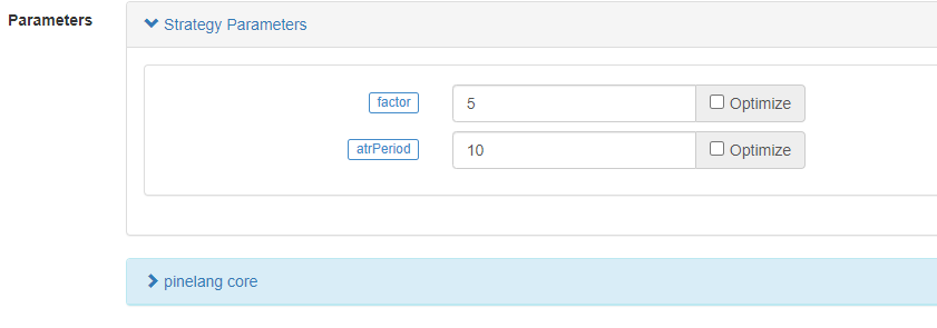
As we can see, the default value on the control is the first parameter of the input function and the input series of functions (here input.int), which are also explained in the previous sections. With these two functions, we can then set the parameters of the ta.supertrend function on the strategy screen. The supertrend function calculates a price data supertrend and a direction data direction. Then use the plot function to draw a chart, note that when drawing the chart, it is based on the direction of the supertrend indicator, only the current direction is drawn. When direction is -1, the current market trend is upward, when direction is 1, the current market trend is downward. So we can see that the plot function draws the chart when the judgment direction is greater than, less than 0.

The next if... else if logic is the judgment of the trading signal. When the expression direction<0 is true, it means that the current market is in the upward stage. At this time, if the price data supertrend in the super trend indicator is higher than the price of the super trend indicator on the two previous BARs (that is, supertrend [2]. Remember that the historical operator refers to the historical data of a variable), it will be used as an entry signal to go long. Remember that? If there is a current position, calling the reverse order function will close the previous position first, and then open the position according to the current trading direction. In addition, even if the condition supertrend>supertrend [2] have not been met, as long as the strategy position_ Size<0 holding short positions, it will trigger strategy. close_ All() function execution to close all positions.

direction > 0 It is the same when it is in the downward trend stage. If there are long positions, all positions will be closed, and then when the condition supertrend<supertrend [3] is met, a short signal will be triggered. Why is it set to [3] to reference the price data of the super trend indicator on the third BAR of the previous number? It may be the intention of the strategy author. After all, the short risk in some markets, such as the contract trading market, is slightly greater than the long risk.

For ta.supertrend Indicator. Are some students interested in how to judge whether the current trend is upward or downward?

In fact, this indicator can also be implemented in the form of custom functions in the Pine language:

pine_supertrend(factor, atrPeriod) =>
	src = hl2
	atr = ta.atr(atrPeriod)
	upperBand = src + factor * atr
	lowerBand = src - factor * atr
	prevLowerBand = nz(lowerBand[1])
	prevUpperBand = nz(upperBand[1])

	lowerBand := lowerBand > prevLowerBand or close[1] < prevLowerBand ? lowerBand : prevLowerBand
	upperBand := upperBand < prevUpperBand or close[1] > prevUpperBand ? upperBand : prevUpperBand
	int direction = na
	float superTrend = na
	prevSuperTrend = superTrend[1]
	if na(atr[1])
		direction := 1
	else if prevSuperTrend == prevUpperBand
		direction := close > upperBand ? -1 : 1
	else
		direction := close < lowerBand ? 1 : -1
	superTrend := direction == -1 ? lowerBand : upperBand
	[superTrend, direction]

This custom function is exactly the same algorithm as the built-in function ta.supertrend, and of course the calculated indicator data is also exactly the same.
As we can see from this custom function algorithm, Pine's built-in super trend indicator is calculated by using the hl2 built-in variable (the highest and lowest prices are added together and then divided by 2, that is, the average of the highest and lowest prices), and then the ATR indicator (volatility) is calculated for a certain period based on the parameter atrPeriod. Then the upper and lower tracks are constructed by using hl2 and ATR.

Update lowerBand and upperBand according to the ternary expressions in the code.

    lowerBand := lowerBand > prevLowerBand or close[1] < prevLowerBand ? lowerBand : prevLowerBand
    upperBand := upperBand < prevUpperBand or close[1] > prevUpperBand ? upperBand : prevUpperBand

lowerBand: lowerBand, used to determine if the upward trend has changed. upperBand: upperBand, used to determine if the downward trend has changed. lowerBand and upperBand are always calculated, only the current trend direction is determined at the end of this custom function.

    else if prevSuperTrend == prevUpperBand
        direction := close > upperBand ? -1 : 1
    else
        direction := close < lowerBand ? 1 : -1

Here it is judged that if the price value of the last BAR on the super trend is prevUpperBand, i.e. the upperBand, it means that the current is a downward trend. At this point, if the close exceeds the upperBand price breakout, the trend is considered to have shifted at this point and converted to an uptrend. The direction variable direction is set to -1 (uptrend). Otherwise it is still set to 1 (downward trend). That's why you see in the super trend strategy if direction < 0 when the signal condition is triggered to go long. When direction > 0, the signal condition is triggered to go short.

    superTrend := direction == -1 ? lowerBand : upperBand
    [superTrend, direction]

Finally, specific Super Trend Indicator price data and direction data are returned based on the direction selection.

Dynamic balancing strategy

/*backtest
start: 2021-03-01 00:00:00
end: 2022-09-08 00:00:00
period: 1h
basePeriod: 15m
exchanges: [{"eid":"Binance","currency":"ETH_USDT"}]
args: [["v_input_1",4374],["v_input_2",3],["v_input_3",300],["ZPrecision",0,358374]]
*/

varip balance = input(50000, "balance")
varip stocks = input(0, "stocks")

maxDiffValue = input(1000, "maxDiffValue")


if balance - close * stocks > maxDiffValue and not barstate.ishistory
    // more balance , open long 
    tradeAmount = (balance - close * stocks) / 2 / close
    strategy.order("long", strategy.long, tradeAmount)
    balance := balance - tradeAmount * close
    stocks := stocks + tradeAmount
    runtime.log("balance:", balance, ", stocks:", stocks, ", tradeAmount:", tradeAmount)

else if close * stocks - balance > maxDiffValue and not barstate.ishistory
    // more stocks , open short 
    tradeAmount = (close * stocks - balance) / 2 / close
    strategy.order("short", strategy.short, tradeAmount)
    balance := balance + tradeAmount * close
    stocks := stocks - tradeAmount
    runtime.log("balance:", balance, ", stocks:", stocks, ", tradeAmount:", tradeAmount)

plot(balance, title="balance value(quoteCurrency)", color=color.red)
plot(stocks*close, title="stocks value(quoteCurrency)", color=color.blue)

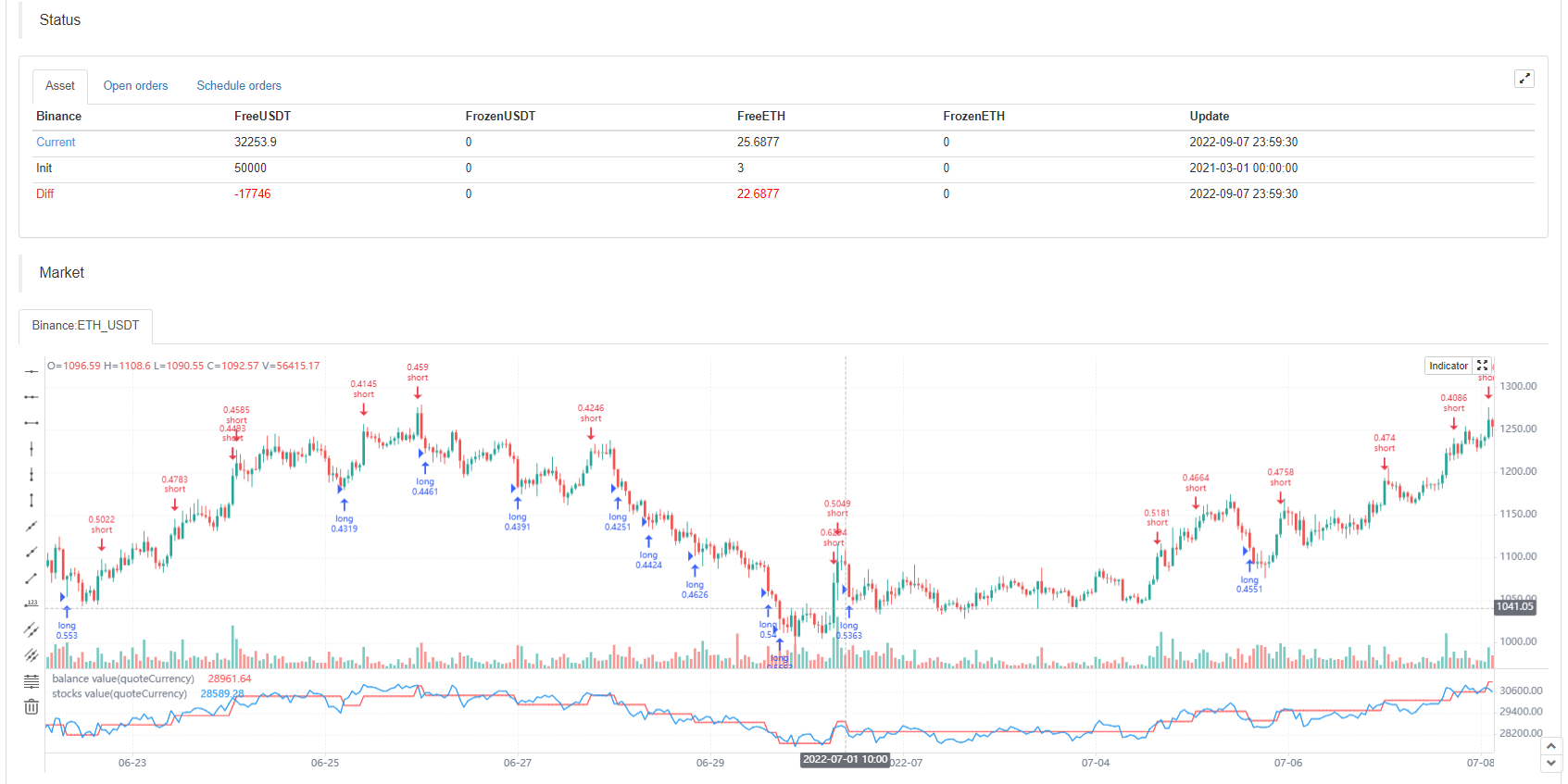
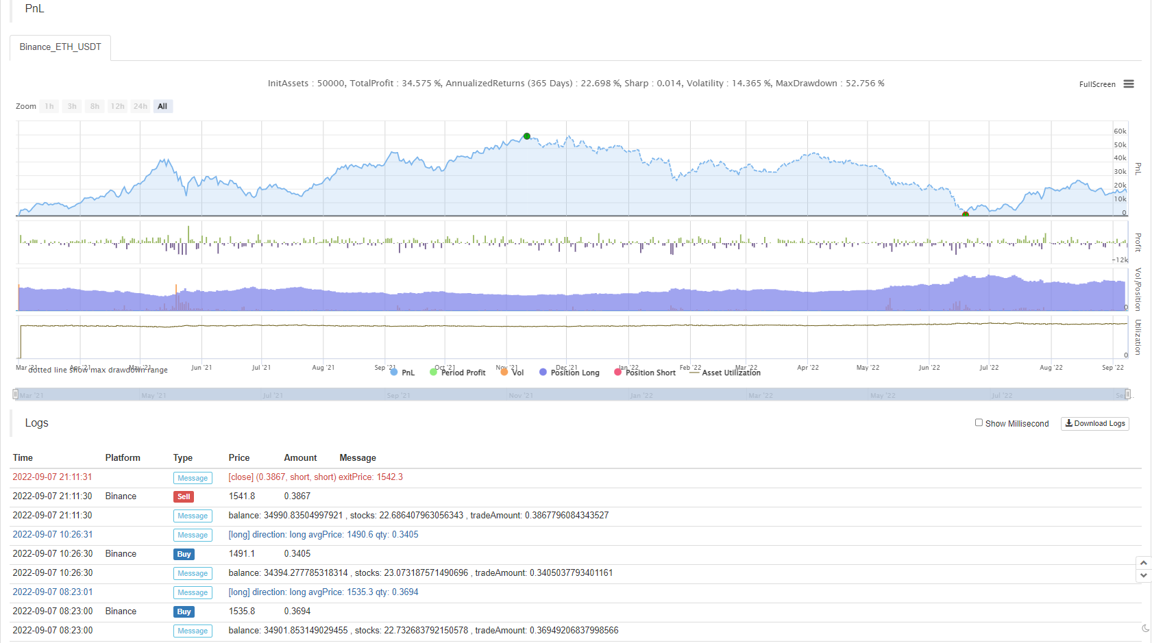
Let's continue with some Pine language strategy design examples, this time we'll look at a dynamic balancing strategy. A dynamic balancing strategy is one that always balances the amount of BaseCurrency and the amount of QuoteCurrency. Whichever asset's relative price increases, the value held in the account increases and the asset is sold. If the relative price of an asset decreases, the value held in the account decreases and the asset is bought. This is known as a dynamic balancing strategy. In fact, the dynamic balance strategy is a kind of grid strategy that performs well in oscillating markets. But in the trend market, it will continue to lose money, we need to wait for the price to return to reduce losses slowly to profit, but the advantage is that the dynamic balancing strategy can always capture the oscillating trend of the market.

The disadvantage, as shown on the backtest chart of this strategy, is that the strategy has a large floating loss during the stage of the general price trend up (or down). So this strategy is fine for spot strategies, but you need to control the risk for futures.

Let's look at the strategy code design:

We use a simplified design that simulates a balance (i.e., the number of QuoteCurrency assets) and stocks (i.e., the number of BaseCurrency assets) balance information in the strategy. We don't read the real number of assets in the account, we simply use the simulated amount to calculate the appropriate buys and sells. Then the key parameter that affects the grid pulled by this dynamic balancing strategy is the maxDiffValue, which is the judgment criterion to carry out the balancing. At the current price, only when the deviation between BaseCurrency and QuoteCurrency exceeds maxDiffValue does the balancing process take place, selling the asset with a high price and buying the asset with a low price to rebalance the asset.

The strategy trading signal trigger must be in the real-time BAR stage, so if judgments in the strategy trading conditions are set with not barstate.ishistory. Buy when the balance value exceeds the stocks value based on the current price calculation. Conversely, a sell operation is performed. After executing the trade statement, the balance and stocks variables are updated and then await the next balance trigger.

The above information of the strategy backtest contains the price of the species at the start time of the strategy backtest, the price is 1458, so I set the parameter balance to: 4374 (1458*3) deliberately, set the parameter stocks to: 3. Let the asset start in balance.

Super Trend Strategy with Tracking Stop Loss and Take Profit

In the previous course, we have learned about the strategy.exit position exit function, of which we did not have an example to explain the tracking stop and take profit function. In this strategy design example, we will use the strategy.exit function to optimize a super trend strategy.

First let's look at the tracking stop-loss and take-profit parameters of the strategy.exit function:

trail_price parameters: The position that triggers the logical action of placing a tracking stop-loss and stop-loss close order (at the position specified by price).
trail_offset parameters: The distance from the highest (when going long) or lowest (when going short) price of a closed position placed after the execution of a tracking stop-loss and take-profit action.
trail_points parameters: Like the trail_price parameter, except that it takes profit points as the specified position.

Is that not easy to understand? It doesn't matter! Let's go through a strategy backtesting scenario to understand, which is actually quite simple.

/*backtest
start: 2022-09-23 00:00:00
end: 2022-09-23 08:00:00
period: 1m
basePeriod: 1m
exchanges: [{"eid":"Binance","currency":"ETH_USDT"}]
args: [["RunMode",1,358374],["ZPrecision",0,358374]]
*/

strategy("test", overlay = true)

varip a = na
varip highPrice = na
varip isTrade = false 
varip offset = 30

if not barstate.ishistory and not isTrade
    strategy.entry("test 1", strategy.long, 1)
    strategy.exit("exit 1", "test 1", 1, trail_price=close+offset, trail_offset=offset)
    a := close + offset
    runtime.log("the price per point is:", syminfo.mintick, ", current close:", close)
    isTrade := true 

if close > a and not barstate.ishistory
    highPrice := na(highPrice) ? close : highPrice
    highPrice := close > highPrice ? close : highPrice

plot(a, "trail_price trigger line")    
plot(strategy.position_size>0 ? highPrice : na, "current highest price")
plot(strategy.position_size>0 ? highPrice-syminfo.mintick*offset : na, "moving stop trigger line")

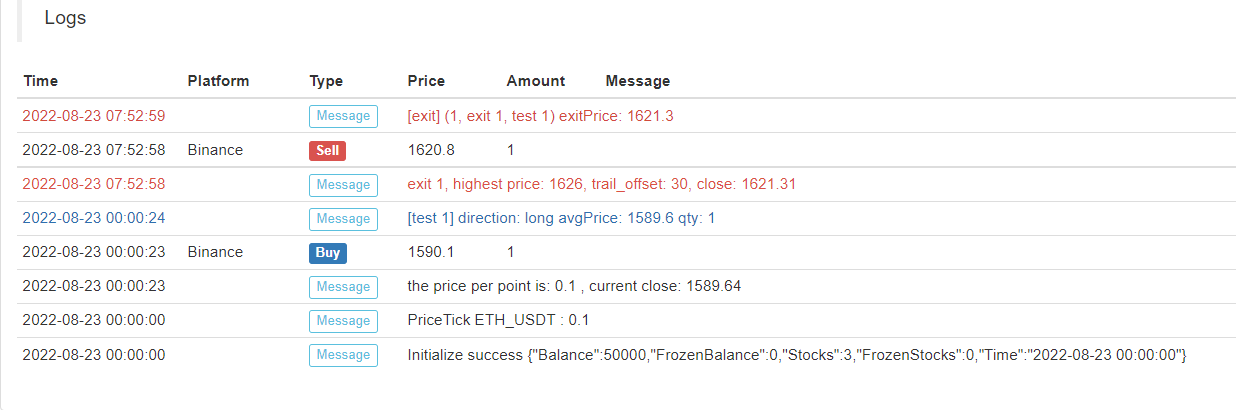
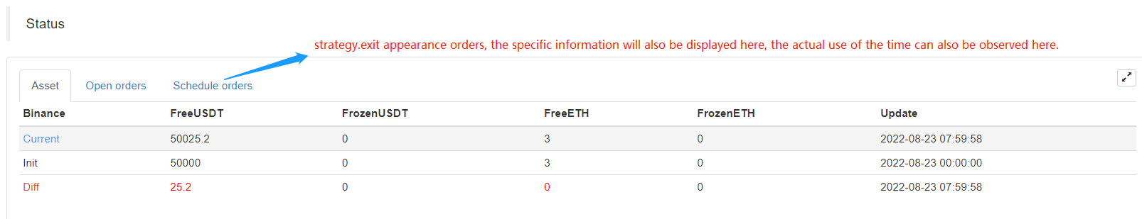
Strategy began to implement the immediate long entry, and then immediately placed a strategy.exit exit order (specified the tracking stop-loss and take-profit parameters), when the price of the market change rose above the trail_price trigger line, the implementation of the trailing stop-loss and take-profit logic, stop-loss and take-profit line (blue) began to follow the highest price dynamic adjustment, the blue line position is the stop-loss and take-profit trigger to close the position, and finally when the market price falls below the blue line that triggers the closure of the position. Combined with the line drawn on the chart, it is very easy to understand.

Then we use this feature to optimize a super trending strategy, we simply assign a strategy.exit exit plan order to the strategy entry order to add this trailing stop-loss and take-profit feature.

if not barstate.ishistory and findOrderIdx("open") >= 0 and state == 1
    trail_price := strategy.position_size > 0 ? close + offset : close - offset
    strategy.exit("exit", "open", 1, trail_price=trail_price, trail_offset=offset)
    runtime.log("the price per point is:", syminfo.mintick, ", current close:", close, "，trail_price：", trail_price)
    state := 2 
    tradeBarIndex := bar_index

Complete strategy code:

/*backtest
start: 2022-05-01 00:00:00
end: 2022-09-27 00:00:00
period: 1d
basePeriod: 5m
exchanges: [{"eid":"Binance","currency":"ETH_USDT"}]
args: [["RunMode",1,358374],["ZPrecision",0,358374]]
*/

varip trail_price = na
varip offset = input(50, "offset")
varip tradeBarIndex = 0
// 0 : idle , 1 current_open , 2 current_close
varip state = 0  

findOrderIdx(idx) =>
    ret = -1 
    if strategy.opentrades == 0 
        ret
    else 
        for i = 0 to strategy.opentrades - 1 
            if strategy.opentrades.entry_id(i) == idx
                ret := i 
                break
        ret

if strategy.position_size == 0 
    trail_price := na 
    state := 0

[superTrendPrice, dir] = ta.supertrend(input(2, "atr coefficient"), input(20, "atr period"))

if ((dir[1] < 0 and dir[2] > 0) or (superTrendPrice[1] > superTrendPrice[2])) and state == 0 and tradeBarIndex != bar_index
    strategy.entry("open", strategy.long, 1)
    state := 1
else if ((dir[1] > 0 and dir[2] < 0) or (superTrendPrice[1] < superTrendPrice[2])) and state == 0 and tradeBarIndex != bar_index
    strategy.entry("open", strategy.short, 1)
    state := 1


// Reverse signal, close all positions
if strategy.position_size > 0 and dir[2] < 0 and dir[1] > 0
    strategy.cancel_all()
    strategy.close_all()
    runtime.log("trend reversal, long positions all closed")
else if strategy.position_size < 0 and dir[2] > 0 and dir[1] < 0
    strategy.cancel_all()
    strategy.close_all()
    runtime.log("trend reversal, short positions all closed")


if not barstate.ishistory and findOrderIdx("open") >= 0 and state == 1
    trail_price := strategy.position_size > 0 ? close + offset : close - offset
    strategy.exit("exit", "open", 1, trail_price=trail_price, trail_offset=offset)
    runtime.log("the price per point is:", syminfo.mintick, ", current close:", close, ", trail_price:", trail_price)
    state := 2 
    tradeBarIndex := bar_index


plot(superTrendPrice, "superTrendPrice", color=dir>0 ? color.red : color.green, overlay=true)

Pine language foundation

Model execution

Time series

Script structure

General structure

Comments

Code

Line break code

Markers and Operators

Markers

Operators

Assignment Operators

Arithmetic Operators

Comparison Operators

Logical Operators

Ternary Operator

Historical Operator

Operator Priority

Variables

Variable Declaration

Condition Structure

if statement

switch statement

Loop Structure

for statement

for ... in statement

while statemnet

Arrays

Arrays Declaration

Read and write elements in an array

Iterate through array elements

Historical data references

Functions for adding and deleting arrays

Array calculation and operation functions commonly used

Functions

Custom Functions

Built-in functions

Trading Functions

Strategy Examples

Super Trend Indicator Strategy

Dynamic balancing strategy

Super Trend Strategy with Tracking Stop Loss and Take Profit

Share this article：

Leave a Reply Cancel reply