Time series data
Time series refers to the data series obtained in a continuous interval of equal time. In quantitative investment, these data are mainly reflected in the price and the movement of the data points of the tracked investment object. For example, for stock prices, the time series data recorded regularly within a specified time period can refer to the following chart, which will give the readers a clearer understanding:
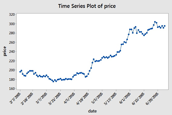
As you can see, the date is on the x-axis, and the price is displayed on the y-axis. In this case, “continuous interval time period” means that the days on the x-axis are separated by 14 days: note the difference between March 7, 2005 and the next point, March 31, 2005, April 5, 2005, and April 19, 2005.
However, when you use time series data, you will often see more than just this kind of data that only contains two columns: date and price. In most cases, you will use five columns of data: data period, opening price, highest price, lowest price, and closing price. This means that if your data period is set to the daily level, the high, open, low and close price changes of the day will be reflected in the data of this time series.
What is Tick data?
Tick data is the most detailed trading data structure in the exchange. It is also an extended form of time series data mentioned above, including: opening price, highest price, lowest price, latest price, trading quantity and turnover. If the transaction data is compared to a river, the Tick data is the data of the river at a certain cross section.
Every action of foreign exchanges will be pushed to the market in real-time, while the domestic exchange checks twice a second. If there are actions in this period, a snapshot will be generated and pushed. In comparison, data push can only be regarded as OnTime at best, not OnTick.
All codes and time series data acquisition in this tutorial will be completed on the FMZ Quant platform.
Tick data on the FMZ Quant
Although the domestic Tick data is not a real Tick, it can be infinitely close to and restore the reality at least by using this data for backtesting. Each tick displays the main parameters of the product in the market at that time, and our code in the real bot is calculated according to the theoretical Tick of twice a second.
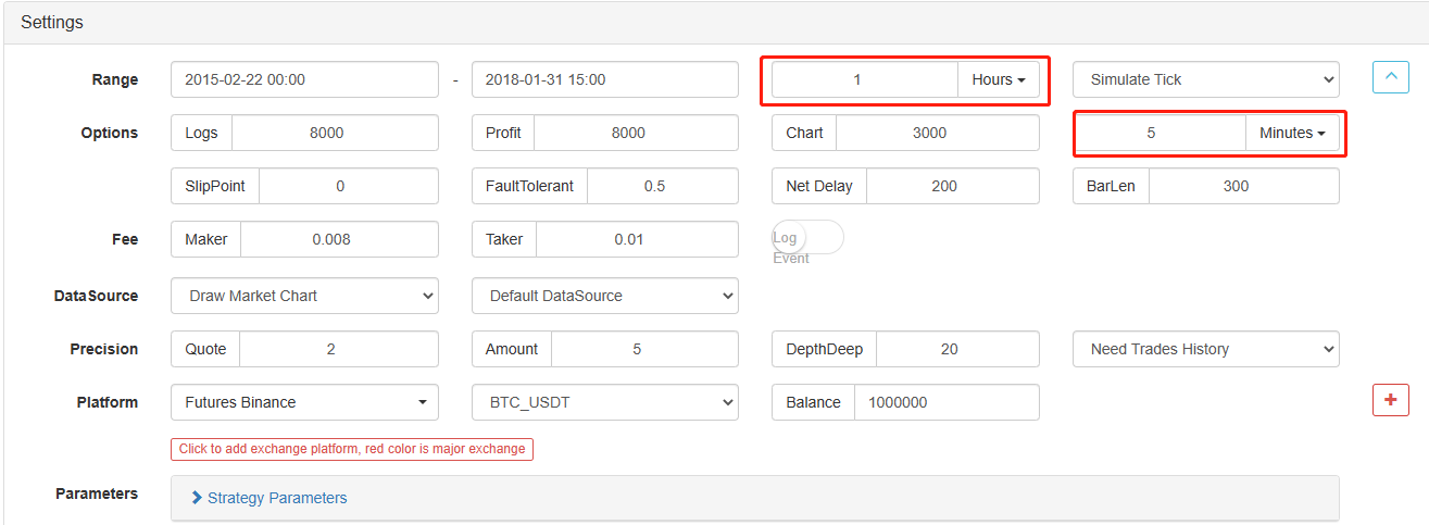
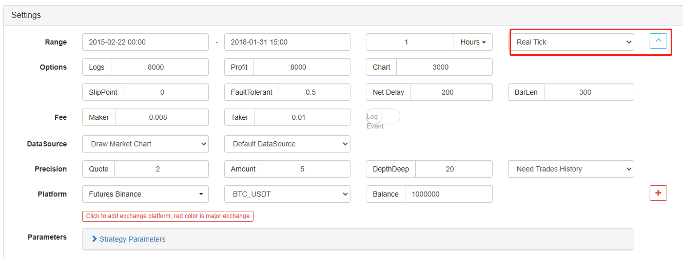
Not only that, on the FMZ Quant, even if the data with a 1-hour period is loaded, the data granularity can still be adjusted, such as adjusting the data granularity to 1 minute. At this moment, the 1-hour K-line is composed of 1-minute data. Of course, the smaller the granularity, the higher the precision. What is more powerful is that if you switch the data to a real bot Tick, you can restore the real bot environment seamlessly. That is, the real data of the Tick Exchange of twice a second.
Now you have learned the basic concepts you need to understand to complete this tutorial. These concepts will come back soon, and you will learn more about them later in this tutorial.
Set up the working environment
Better tools make good work. We need to deploy a docker on the FMZ Quant platform first. With regard to the concept of a docker, readers with programming experience can imagine it as an officially packaged Docker system, which has encapsulated the public API interfaces of various mainstream exchanges and the technical details of strategy writing and backtesting. The original intention of establishing this system is to make quantitative traders focus on strategy writing and design when using the FMZ Quant platform. These technical details are presented to strategy writers in an encapsulated form to save them a lot of time and effort.
- Deployment of the docker system of the FMZ Quant platform
There are two methods to deploy a docker:
Method A: Users can rent or purchase servers themselves and deploy them on various cloud computing platforms, such as AWS, Alibaba Cloud, Digital Ocean and Google Cloud. The advantage is that both strategy security and system security are guaranteed. For the FMZ Quant platform, users are encouraged to use this method. The distributed deployment eliminates the hidden danger of server attacks (whether it is the customer or the platform itself).
For more information on this part, readers can refer to: https://www.fmz.com/bbs-topic/2848.
Method B: Use the public server of the FMZ Quant platform for deployment, the platform provides four locations for deployment in Hong Kong, Singapore, Japan and Eastern US. Users can deploy according to the location of the exchange they want to trade and the principle of proximity. The advantage of this aspect is that it is simple and easy to complete with one click, which is especially suitable for beginner users. It does not need to know many things about purchasing Linux servers, and it also saves time and energy from learning Linux commands. The price is relatively cheap. For users with small funds, the platform recommends using this deployment method.
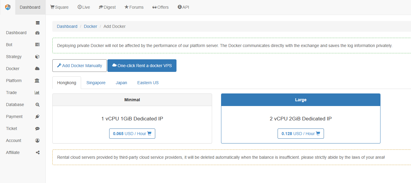
For beginners’ understanding, this article will adopt method B.
The specific operations are: log in to FMZ.COM, click Dashboard, Docker, and click One-click Rent a docker VPS to rent the docker.
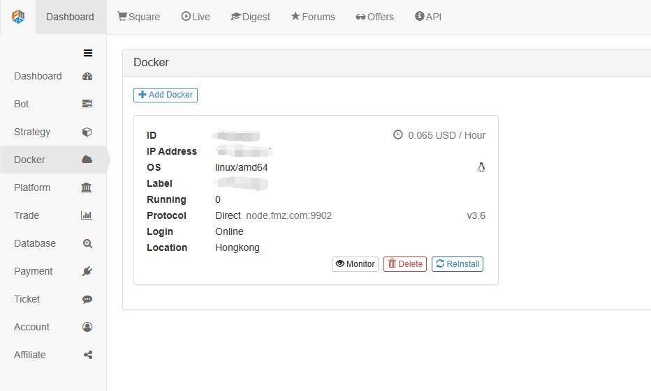
Enter the password, as shown below after successful deployment:
- The relationship between the concept of robot system and the docker
As mentioned above, the docker is like a docker system, and a docker system is like a set of standards. We have deployed this set of standards. Next, we need to generate an “instance” for this standard, which is a robot.
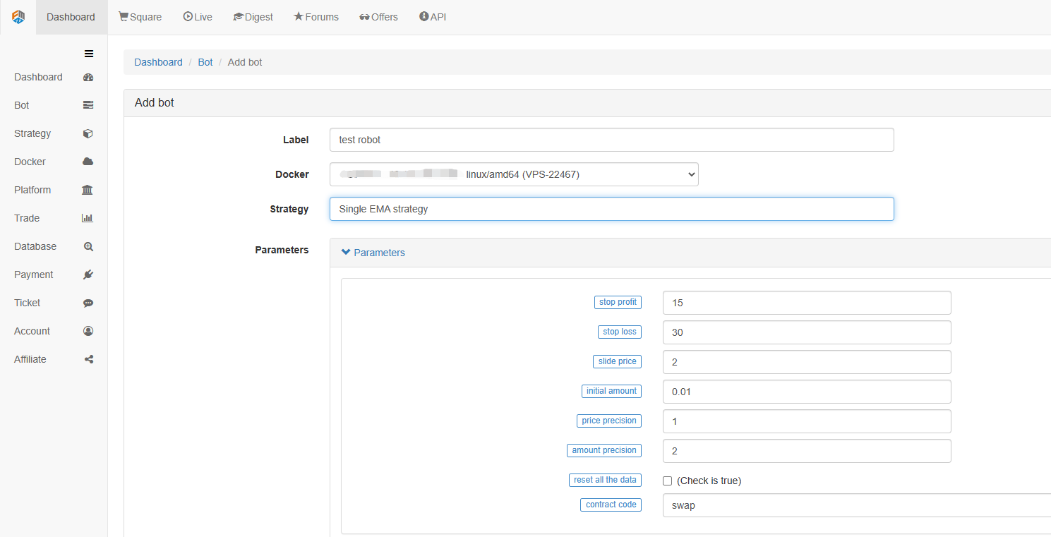
Creating a robot is very simple. After deploying the docker, click the Bot column on the left, click Add bot, fill in a name in the tag name, and select the docker just deployed. The parameters and K-line period below can be set according to the specific situation, mainly in coordination with the trading strategy.
So far, our work environment has been built. It can be seen that it is very simple and effective, and each function performs its own duties. Next, we will begin to write a quantitative strategy.
Implement a simple EMA strategy in Python
We mentioned the concepts of time series data and Tick data above. Next, we use a simple EMA strategy to link the two concepts.
- The basic principle of EMA strategy
Through a slow period EMA, such as the 7-day EMA, and a fast period EMA, such as the 3-day EMA. They are applied to the same K-line chart. When the fast period EMA crosses over the slow period EMA, we call it Golden Cross; When the slow period EMA goes down through the fast period EMA, we call it Bearish Crossover.
The basis for opening a position is to open long positions with a Golden Cross, and open short positions with a Bearish Crossover. The reason for closing positions is the same.
Let’s open FMZ.COM, log in to the account, Dashboard, Strategy library, and create a new strategy. Select Python in the strategy writing language in the upper left corner. The following is the code of this strategy. Each line has detailed comments. Please take your time to understand. This strategy is not a real bot strategy. Don’t experiment with real money. The main purpose is to give you a general idea of strategy writing and a template for learning.
import types # Import the Types module library, which is designed to handle the various data types that will be used in the code.

def main(): # The main function, where the strategy logic begins.
    STATE_IDLE = -1 # Mark position status variables
    state = STATE_IDLE # Mark the current position status
    initAccount = ext.GetAccount() # The spot digital currency trading class library (python version) is used here. Remember to check it when writing the strategy to obtain the initial account information.
    while True: # Enter the loop
        if state == STATE_IDLE : # Here begins the logic of opening positions.
            n = ext.Cross(FastPeriod,SlowPeriod) # The indicator crossover function is used here, for details please see: https://www.fmz.com/strategy/21104.
            if abs(n) >= EnterPeriod : # If n is greater than or equal to the market entry observation period, the market entry observation period here is to prevent positions from being opened indiscriminately as soon as the market opens.
                opAmount = _N(initAccount.Stocks * PositionRatio,3) # Opening position quantity, for the usage of _N, please check the official API documentation.
                Dict = ext.Buy(opAmount) if n > 0 else ext.Sell(opAmount) # Create a variable to store the open position status and execute the open position operation.
                if Dict :  # Check the dict variable and prepare for the following log output.
                    opAmount = Dict['amount']
                    state = PD_LONG if n > 0 else PD_SHORT # Both PD_LONG and PD_SHORT are global constants used to represent long and short positions, respectively.
                    Log("Details of opening positions",Dict,"Cross-period",n) # Log information
        else: # Here begins the logic of closing positions.
            n = ext.Cross(ExitFastPeriod,ExitSlowPeriod) # The indicator crossover function.
            if abs(n) >= ExitPeriod and ((state == PD_LONG and n < 0) or (state == PD_SHORT and n > 0)) : # If the market exit observation period has passed and the current account status is in the position status, then you can determine the Golden Cross or Bearish Crossover.
                nowAccount = ext.GetAccount() # Refresh and get account information again.
                Dict2 = ext.Sell(nowAccount.Stocks - initAccount.Stocks) if state == PD_LONG else ext.Buy(initAccount.Stocks - nowAccount.Stocks) # The logic of closing a position is to close the long position if it is a long position and close the short position if it is a short position.
                state = STATE_IDLE # Mark the position status after closing positions.
                nowAccount = ext.GetAccount() # Refresh and get account information again.
                LogProfit(nowAccount.Balance - initAccount.Balance,'money:',nowAccount.Balance,'currency:',nowAccount.Stocks,'The details of closing positions',Dict2,'Cross-over period:',n) # Log information
        Sleep(Interval * 1000) # Pause the loop for one second to prevent the account from being restricted due to too fast API access frequency.
- Backtesting of EMA strategy
On the strategy editing page, we have finished writing the strategy. Next, we need to backtest the strategy to see how it performs in the historical market. Backtesting plays an important role in any quantitative strategy development, but it can only be used as an important reference. Backtesting is not equal to profit guarantee, because the market is changing constantly, and backtesting is just an act of hindsight, which still belongs to the category of induction, the market is deductive.
Click the backtest, you can see that there are many adjustable parameters, which can be modified directly. For the future, the strategy is more and more complex, and the parameters are more and more. This method of modification can help users avoid the trouble of modifying code one by one, which is convenient, fast, and clear.
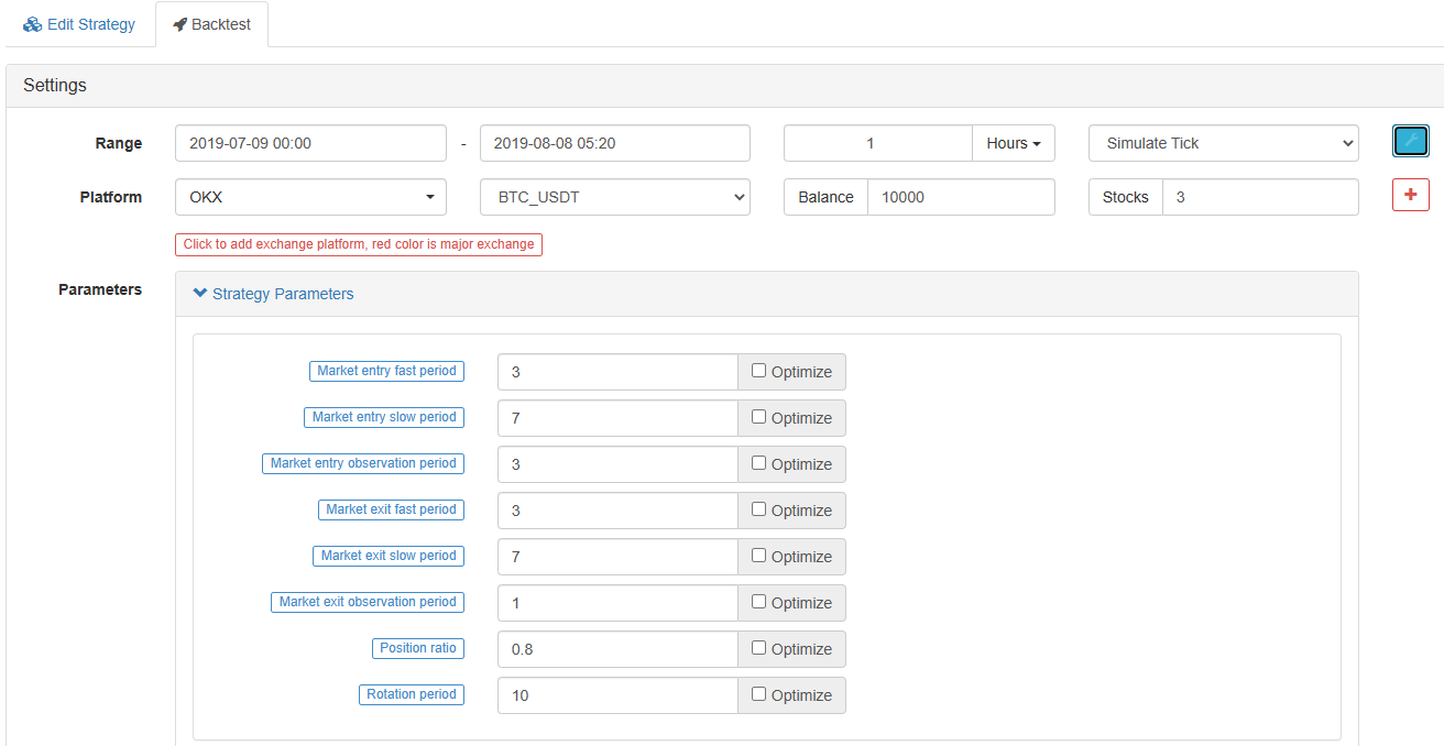
The following optimization options can optimize the set parameters automatically. The system will try various optimal parameters to help strategy developers find the optimal choice.
From the examples above, we can see that the basis of quantitative trading is through the analysis of time series data and the backtesting interaction of tick data. No matter how complex the logic is, it cannot be separated from these two basic elements. The difference is just the difference in dimensions. For example, high-frequency transactions require more detailed data aspects and more time series data. Another example is arbitrage trading, which requires a lot of data from the backtest sample. It may require continuous in-depth data of two trading objects for more than ten years to find out the statistical results of their interest margin expansion and reduction. In future articles, I will introduce high-frequency trading and arbitrage trading strategies one after another. Please look forward to it.