Introduction to Dual Thrust trading algorithm
The Dual Thrust trading algorithm is a famous quantitative trading strategy developed by Michael Chalek. It is usually used in futures, foreign exchange and stock markets. The concept of Dual Thrust is a typical breakthrough trading system. It uses the “double thrust” system to build an updated backtracking period based on historical prices, which theoretically makes it more stable in any given period.
In this article, we give the detailed logic details of this strategy and show how to implement this algorithm on the FMZ Quant platform. First of all, we need to select the historical price of the subject matter to be traded. This range is calculated based on the closing price, the highest price and the lowest price of the last N days. When the market moves a certain range from the opening price, open the position.
We tested this strategy with a single trading pair under two common market conditions, namely, trend market and shock market. The results showed that the momentum trading system works better in the trend market and it will trigger some invalid trading signals in the volatile market. In the interval market, we can adjust parameters to obtain better returns. As a comparison of individual reference trading targets, we also tested the domestic commodity futures market. The result showed that the strategy is better than the average performance.
DT strategy principle
Its logical prototype is a common intraday trading strategy. The opening range breakthrough strategy is based on today’s opening price plus or minus a certain percentage of yesterday’s range to determine the upper and bottom tracks. When the price crossovers the upper track, it will open its position to buy, and when it breaks the bottom track, it will open its position to go short.
Principle of strategy
- After the closing, two values are calculated: the highest price – the closing price, and the closing price – the lowest price. Then take the larger of the two values and multiply the value by 0.7. Let’s call it the value K, which we call the trigger value.
- After the market opens the next day, record the opening price, and buy immediately when the price exceeds (opening price + trigger value), or sell short positions when the price is lower than (opening price – trigger value).
- This strategy has no obvious stop loss. This system is a reverse system, that is, if there is a short position order when the price exceeds (opening price + trigger value), it will send two buying orders (one closes the wrong position, the other opens the right position). For the same reason, if the price of a long position is lower than (opening price – trigger value), it will send two selling orders.
Mathematical expression of DT strategy
Range = maximum (HH-LC, HC-LL)
The calculation method of long position signal is:
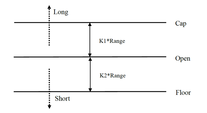
cap = open + K1 × Rangecap = open + K1 × Range
The calculation method of short position signal is:
floor = open – K2 × Rangefloor = open – K2 × Range
Where K1 and K2 are parameters. When K1 is greater than K2, long position signal is triggered, and vice versa. For demonstration, we choose K1=K2=0.5. In actual transactions, we can still use historical data to optimize these parameters or adjust parameters according to market trends. If you are bullish, K1 should be less than K2. If you are bearish, K1 should be greater than K2.
The system is a reversal system. Therefore, if investors hold short positions when the price crossovers the upper track, they should close the short positions before opening long positions. If an investor holds a long position when the price breaks the bottom track, they should close the long position before opening a new short position.
Improvement of DT strategy:
In the range setting, the four price points (high, open, low and close) of the previous N days are introduced to make the range relatively stable in a certain period, which can be applied to daily trend tracking.
The trigger conditions of opening long and short positions of the strategy, considering the asymmetric range, the reference range of long and short transactions should select different number of periods, which can also be determined by parameters K1 and K2. When K1 < K2, the long position signal is relatively easy to be triggered, while when K1 > K2, the short position signal is relatively easy to be triggered.
Therefore, when using this strategy, on the one hand, you can refer to the best parameters of historical data backtesting. On the other hand, you can adjust K1 and K2 in stages according to your judgment of the future or other major period technical indicators.
This is a typical trading method of waiting for signals, entering the market, arbitrage, and then leaving the market, but the effect is excellent.
Deploy DT strategy on the FMZ Quant platform
We open FMZ.COM, log in to the account, click the Dashboard, and deploy the docker and robot.
Please refer to my previous article on how to deploy a docker and robot: https://www.fmz.com/bbs-topic/9864.
Readers who want to purchase their own cloud computing server to deploy dockers can refer to this article: https://www.fmz.com/digest-topic/5711.
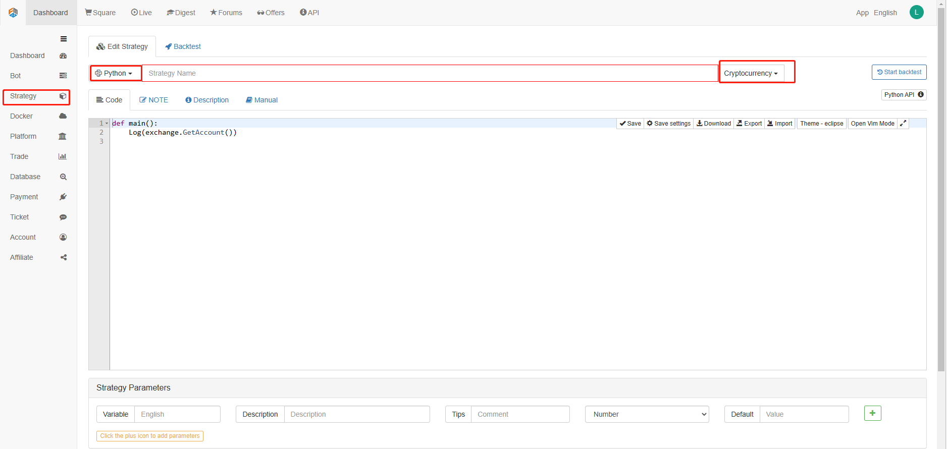
Next, we click on the Strategy Library in the left column and click on Add strategy.
Remember to select the programming language as Python in the upper right corner of the strategy editing page, as shown in the figure:
Next, we will write Python code into the code editing page. The following code has very detailed line-by-line comments, you can take your time to understand.
We will use OKCoin futures to test the strategy:
import time # Here we need to introduce the time library that comes with python, which will be used later in the program.

class Error_noSupport(BaseException): # We define a global class named ChartCfg to initialize the strategy chart settings. Object has many attributes about the chart function. Chart library: HighCharts.
    def __init__(self): # log out prompt messages
        Log("Support OKCoin Futures only! #FF0000")

class Error_AtBeginHasPosition(BaseException):
    def __init__(self):
        Log("Start with a futures position! #FF0000")

ChartCfg = {
    '__isStock': True, # This attribute is used to control whether to display a single control data series (you can cancel the display of a single data series on the chart). If you specify __isStock: false, it will be displayed as a normal chart.
    'title': { # title is the main title of the chart
        'text': 'Dual Thrust upper and bottom track chart' # An attribute of the title text is the text of the title, here set to 'Dual Thrust upper and bottom track chart' the text will be displayed in the title position.
    },
    'yAxis': { # Settings related to the Y-axis of the chart coordinate.
        'plotLines': [{ # Horizontal lines on the Y-axis (perpendicular to the Y-axis), the value of this attribute is an array, i.e. the setting of multiple horizontal lines.
            'value': 0, # Coordinate value of horizontal line on Y-axis
            'color': 'red', # Color of horizontal line
            'width': 2, # Line width of horizontal line
            'label': {  # Labels on the horizontal line
                'text': 'Upper track', # Text of the label
                'align': 'center' # The display position of the label, here set to center (i.e.: 'center')
            },
        }, {       # The second horizontal line ([{...} , {...}] the second element in the array)
            'value': 0, # Coordinate value of horizontal line on Y-axis
            'color': 'green', # Color of horizontal line
            'width': 2,  # Line width of horizontal line
            'label': { # Label
                'text': 'bottom track',
                'align': 'center'
            },
        }]
    },
    'series': [{ # Data series, that is, data used to display data lines, K-lines, tags, and other contents on the chart. It is also an array whose first index is 0.
        'type': 'candlestick', # Type of data series with index 0: 'candlestick' indicates a K-line chart.
        'name': 'Current period',  # Name of the data series
        'id': 'primary', # The ID of the data series, which is used for the related settings of the next data series.
        'data': []  # An array of data series to store specific K-line data
    }, {
        'type': 'flags',  # Data series, type: 'flags', display labels on the chart, indicating going long and going short. Index is 1.
        'onSeries': 'primary',  # This attribute indicates that the label is displayed on id 'primary'.
        'data': []    # The array that holds the label data.
    }]
}

STATE_IDLE = 0  # Status constants, indicating idle
STATE_LONG = 1 # Status constants, indicating long positions
STATE_SHORT = 2 # Status constants, indicating short positions
State = STATE_IDLE # Indicates the current program status, assigned as idle initially

LastBarTime = 0  # The time stamp of the last column of the K-line (in milliseconds, 1000 milliseconds is equal to 1 second, and the timestamp is the number of milliseconds from January 1, 1970 to the present time is a large positive integer).
UpTrack = 0   # Upper track value
BottomTrack = 0 # Bottom track value
chart = None # It is used to accept the chart control object returned by the Chart API function. Use this object (chart) to call its member function to write data to the chart.
InitAccount = None # Initial account status
LastAccount = None # Latest account status
Counter = { # Counters for recording profit and loss counts
    'w': 0, # Number of wins
    'l': 0  # Number of losses
}

def GetPosition(posType):  # Define a function to store account position information
    positions = exchange.GetPosition() # exchange.GetPosition() is the FMZ Quant official API. For its usage, please refer to the official API document: https://www.fmz.com/api.
    return [{'Price': position['Price'], 'Amount': position['Amount']} for position in positions if position['Type'] == posType] # Return to various position information

def CancelPendingOrders(): # Define a function specifically for withdrawing orders
    while True: # Loop check
        orders = exchange.GetOrders() # If there is a position
        [exchange.CancelOrder(order['Id']) for order in orders if not Sleep(500)] # Withdrawal statement
        if len(orders) == 0: # Logical judgment
            break

def Trade(currentState,nextState): # Define a function to determine the order placement logic.
    global InitAccount,LastAccount,OpenPrice,ClosePrice # Define the global scope
    ticker = _C(exchange.GetTicker) # For the usage of _C, please refer to: https://www.fmz.com/api.
    slidePrice = 1 # Define the slippage value
    pfn = exchange.Buy if nextState == STATE_LONG else exchange.Sell # Buying and selling judgment logic
    if currentState != STATE_IDLE: # Loop start
        Log(_C(exchange.GetPosition)) # Log information
        exchange.SetDirection("closebuy" if currentState == STATE_LONG else "closesell") # Adjust the order direction, especially after placing the order.
        while True:
            ID = pfn( (ticker['Last'] - slidePrice) if currentState == STATE_LONG else (ticker['Last'] + slidePrice), AmountOP) # Price limit order, ID=pfn (- 1, AmountOP) is the market price order, ID=pfn (AmountOP) is the market price order.
            Sleep(Interval) # Take a break to prevent the API from being accessed too often and your account being blocked.
            Log(exchange.GetOrder(ID)) # Log information
            ClosePrice = (exchange.GetOrder(ID))['AvgPrice'] # Set the closing price
            CancelPendingOrders() # Call the withdrawal function
            if len(GetPosition(PD_LONG if currentState == STATE_LONG else PD_SHORT)) == 0: # Order withdrawal logic
                break
        account = exchange.GetAccount() # Get account information
        if account['Stocks'] > LastAccount['Stocks']: # If the current account currency value is greater than the previous account currency value.
            Counter['w'] += 1 # In the profit and loss counter, add one to the number of profits.
        else:
            Counter['l'] += 1 # Otherwise, add one to the number of losses.
        Log(account) # log information
        LogProfit((account['Stocks'] - InitAccount['Stocks']),"Return rates:", ((account['Stocks'] - InitAccount['Stocks']) * 100 / InitAccount['Stocks']),'%')
        Cal(OpenPrice,ClosePrice)
        LastAccount = account

    exchange.SetDirection("buy" if nextState == STATE_LONG else "sell") # The logic of this part is the same as above and will not be elaborated.
    Log(_C(exchange.GetAccount))
    while True:
        ID = pfn( (ticker['Last'] + slidePrice) if nextState == STATE_LONG else (ticker['Last'] - slidePrice), AmountOP)
        Sleep(Interval)
        Log(exchange.GetOrder(ID))
        CancelPendingOrders()
        pos = GetPosition(PD_LONG if nextState == STATE_LONG else PD_SHORT)
        if len(pos) != 0:
            Log("Average price of positions",pos[0]['Price'],"Amount:",pos[0]['Amount'])
            OpenPrice = (exchange.GetOrder(ID))['AvgPrice']
            Log("now account:",exchange.GetAccount())
            break

def onTick(exchange): # The main function of the program, within which the main logic of the program is processed.
    global LastBarTime,chart,State,UpTrack,DownTrack,LastAccount # Define the global scope
    records = exchange.GetRecords() # For the usage of exchange.GetRecords(), please refer to: https://www.fmz.com/api.
    if not records or len(records) <= NPeriod: # Judgment statements to prevent accidents.
        return
    Bar = records[-1] # Take the penultimate element of records K-line data, that is, the last bar.
    if LastBarTime != Bar['Time']:
        HH = TA.Highest(records, NPeriod, 'High')  # Declare the HH variable, call the TA.Highest function to calculate the maximum value of the highest price in the current K-line data NPeriod period and assign it to HH.
        HC = TA.Highest(records, NPeriod, 'Close') # Declare the HC variable to get the maximum value of the closing price in the NPeriod period.
        LL = TA.Lowest(records, NPeriod, 'Low') # Declare the LL variable to get the minimum value of the lowest price in the NPeriod period.
        LC = TA.Lowest(records, NPeriod, 'Close') # Declare LC variable to get the minimum value of the closing price in the NPeriod period. For specific TA-related applications, please refer to the official API documentation.

        Range = max(HH - LC, HC - LL)  # Calculate the range
        UpTrack = _N(Bar['Open'] + (Ks * Range))  # The upper track value is calculated based on the upper track factor Ks of the interface parameters such as the opening price of the latest K-line bar.
        DownTrack = _N(Bar['Open'] - (Kx * Range)) # Calculate the down track value
        if LastBarTime > 0: # Because the value of LastBarTime initialization is set to 0, LastBarTime>0 must be false when running here for the first time. The code in the if block will not be executed, but the code in the else block will be executed.
            PreBar = records[-2] # Declare a variable means "the previous Bar" assigns the value of the penultimate Bar of the current K-line to it.
            chart.add(0, [PreBar['Time'], PreBar['Open'], PreBar['High'], PreBar['Low'], PreBar['Close']], -1) # Call the add function of the chart icon control class to update the K-line data (use the penultimate bar of the obtained K-line data to update the last bar of the icon, because a new K-line bar is generated).
        else:  # For the specific usage of the chart.add function, see the API documentation and the articles in the forum. When the program runs for the first time, it must execute the code in the else block. The main function is to add all the K-lines obtained for the first time to the chart at one time.
            for i in range(len(records) - min(len(records), NPeriod * 3), len(records)): # Here, a for loop is executed. The number of loops uses the minimum of the K-line length and 3 times the NPeriod, which can ensure that the initial K-line will not be drawn too much and too long. Indexes vary from large to small.
                b = records[i] # Declare a temporary variable b to retrieve the K-line bar data with the index of records.length - i for each loop.
                chart.add(0,[b['Time'], b['Open'], b['High'], b['Low'], b['Close']]) # Call the chart.add function to add a K-line bar to the chart. Note that if the last parameter of the add function is passed in -1, it will update the last Bar (column) on the chart. If no parameter is passed in, it will add Bar to the last. After executing the loop of i=2 (i-- already, now it's 1), it will trigger i > 1 for false to stop the loop. It can be seen that the code here only processes the bar of records.length - 2, and the last Bar is not processed.
        chart.add(0,[Bar['Time'], Bar['Open'], Bar['High'], Bar['Low'], Bar['Close']]) # Since the two branches of the above if do not process the bar of records.length - 1, it is processed here. Add the latest Bar to the chart.
        ChartCfg['yAxis']['plotLines'][0]['value'] = UpTrack  # Assign the calculated upper track value to the chart object (different from the chart control object chart) for later display.
        ChartCfg['yAxis']['plotLines'][1]['value'] = DownTrack # Assign lower track value
        ChartCfg['subtitle'] = { # Set subtitle
            'text': 'upper tarck' + str(UpTrack) + 'down track' + str(DownTrack) # Subtitle text setting. The upper and down track values are displayed on the subtitle.
        }
        chart.update(ChartCfg) # Update charts with chart class ChartCfg.
        chart.reset(PeriodShow) # Refresh the PeriodShow variable set according to the interface parameters, and only keep the K-line bar of the number of PeriodShow values.

        LastBarTime = Bar['Time'] # The timestamp of the newly generated Bar is updated to LastBarTime to determine whether the last Bar of the K-line data acquired in the next loop is a newly generated one.
    else: # If LastBarTime is equal to Bar.Time, that is, no new K-line Bar is generated. Then execute the code in {..}.
        chart.add(0,[Bar['Time'], Bar['Open'], Bar['High'], Bar['Low'], Bar['Close']], -1) # Update the last K-line bar on the chart with the last Bar of the current K-line data (the last Bar of the K-line, i.e. the Bar of the current period, is constantly changing).
    LogStatus("Price:", Bar["Close"], "up:", UpTrack, "down:", DownTrack, "wins:", Counter['w'], "losses:", Counter['l'], "Date:", time.time()) # The LogStatus function is called to display the data of the current strategy on the status bar.
    msg = "" # Define a variable msg.
    if State == STATE_IDLE or State == STATE_SHORT: # Judge whether the current state variable State is equal to idle or whether State is equal to short position. In the idle state, it can trigger long position, and in the short position state, it can trigger a long position to be closed and sell the opening position.
        if Bar['Close'] >= UpTrack: # If the closing price of the current K-line is greater than the upper track value, execute the code in the if block.
            msg = "Go long, trigger price:" + str(Bar['Close']) + "upper track" + str(UpTrack) # Assign a value to msg and combine the values to be displayed into a string.
            Log(msg) # message
            Trade(State, STATE_LONG) # Call the Trade function above to trade.
            State = STATE_LONG # Regardless of opening long positions or selling the opening position, the program status should be updated to hold long positions at the moment.
            chart.add(1,{'x': Bar['Time'], 'color': 'red', 'shape': 'flag', 'title': 'long', 'text': msg}) # Add a marker to the corresponding position of the K-line to show the open long position.

    if State == STATE_IDLE or State == STATE_LONG: # The short direction is the same as the above, and will not be repeated. The code is exactly the same.
        if Bar['Close'] <= DownTrack:
            msg = "Go short, trigger price:" + str(Bar['Close']) + "down track" + str(DownTrack)
            Log(msg)
            Trade(State, STATE_SHORT)
            State = STATE_SHORT
            chart.add(1,{'x': Bar['Time'], 'color': 'green', 'shape': 'circlepin', 'title': 'short', 'text': msg})

OpenPrice = 0 # Initialize OpenPrice and ClosePrice
ClosePrice = 0
def Cal(OpenPrice, ClosePrice): # Define a Cal function to calculate the profit and loss of the strategy after it has been run.
    global AmountOP,State
    if State == STATE_SHORT:
        Log(AmountOP,OpenPrice,ClosePrice,"Profit and loss of the strategy:", (AmountOP * 100) / ClosePrice - (AmountOP * 100) / OpenPrice, "Currencies, service charge:", - (100 * AmountOP * 0.0003), "USD, equivalent to:", _N( - 100 * AmountOP * 0.0003/OpenPrice,8), "Currencies")
        Log(((AmountOP * 100) / ClosePrice - (AmountOP * 100) / OpenPrice) + (- 100 * AmountOP * 0.0003/OpenPrice))
    if State == STATE_LONG:
        Log(AmountOP,OpenPrice,ClosePrice,"Profit and loss of the strategy:", (AmountOP * 100) / OpenPrice - (AmountOP * 100) / ClosePrice, "Currencies, service charge:", - (100 * AmountOP * 0.0003), "USD, equivalent to:", _N( - 100 * AmountOP * 0.0003/OpenPrice,8), "Currencies")
        Log(((AmountOP * 100) / OpenPrice - (AmountOP * 100) / ClosePrice) + (- 100 * AmountOP * 0.0003/OpenPrice))

def main(): # The main function of the strategy program. (entry function)
    global LoopInterval,chart,LastAccount,InitAccount # Define the global scope
    if exchange.GetName() != 'Futures_OKCoin':  # Judge if the name of the added exchange object (obtained by the exchange.GetName function) is not equal to 'Futures_OKCoin', that is, the object added is not OKCoin futures exchange object.
        raise Error_noSupport # Throw an exception
    exchange.SetRate(1) # Set various parameters of the exchange.
    exchange.SetContractType(["this_week","next_week","quarter"][ContractTypeIdx])  # Determine which specific contract to trade.
    exchange.SetMarginLevel([10,20][MarginLevelIdx]) # Set the margin rate, also known as leverage.

    if len(exchange.GetPosition()) > 0: # Set up fault tolerance mechanism.
        raise Error_AtBeginHasPosition
    CancelPendingOrders()
    InitAccount = LastAccount = exchange.GetAccount()
    LoopInterval = min(1,LoopInterval)
    Log("Trading platforms:",exchange.GetName(), InitAccount)
    LogStatus("Ready...")

    LogProfitReset()
    chart = Chart(ChartCfg)
    chart.reset()

    LoopInterval = max(LoopInterval, 1)
    while True: # Loop the whole transaction logic and call the onTick function.
        onTick(exchange)
        Sleep(LoopInterval * 1000) # Take a break to prevent the API from being accessed too frequently and the account from being blocked.
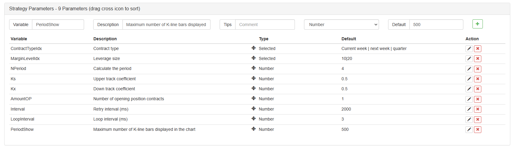
After writing the code, please note that we haven’t finished the whole strategy. Next, we need to add the parameters used in the strategy to the strategy editing page. The method of adding is very simple. Just click the plus sign at the bottom of the strategy writing dialog box to add one by one.
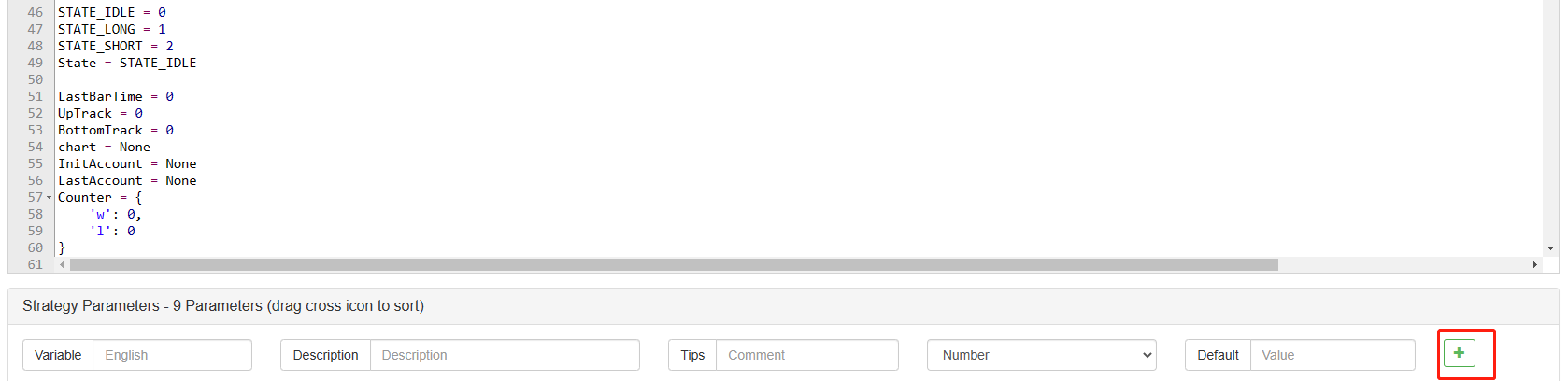
Content to be added:
So far, we have finally completed the writing of the strategy. Next, let’s start backtesting the strategy.
Strategy backtesting
After writing the strategy, the first thing we need to do is to backtest it to see how it behaves in the historical data. But please note that the result of the backtest is not equal to the prediction of the future. The backtest can only be used as a reference to consider the effectiveness of our strategy. Once the market changes and the strategy begins to have great losses, we should find the problem in time, and then change the strategy to adapt to the new market environment, such as the threshold mentioned above. If the strategy has a loss greater than 10%, we should immediately stop the operation of the strategy, and then find the problem. We can start with adjusting the threshold.
Click backtest in the strategy editing page. On the backtest page, the adjustment of parameters can be carried out conveniently and quickly according to different needs. Especially for the strategy with complex logic and many parameters, no need to go back to the source code and modify it one by one.
The backtest time is the latest six months. Click Add OKCoin Futures exchange and select BTC trading target.
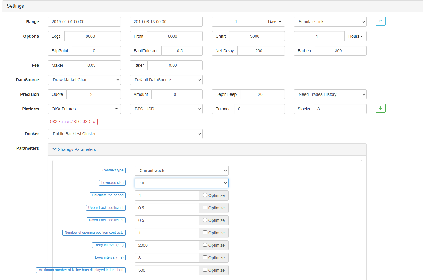
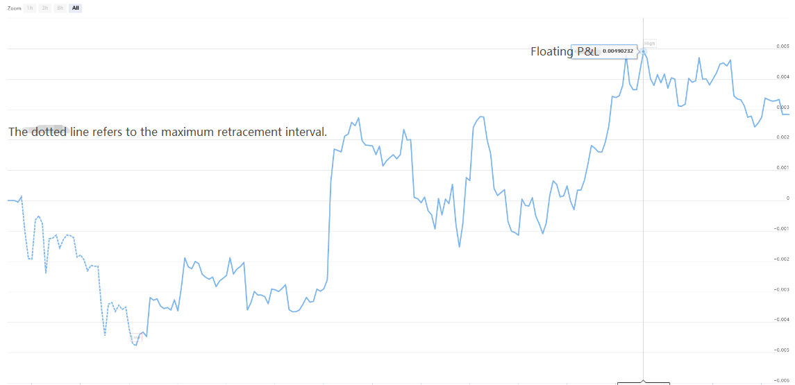
It can be seen that the strategy has reaped good returns in the last six months due to the very good unilateral trend of BTC.

If you have any questions, you can leave a message at https://www.fmz.com/bbs, whether it is about the strategy or the technology of the platform, the FMZ Quant platform has professionals ready to answer your questions.