Bayesian statistics is a powerful discipline in the field of mathematics, with wide applications in many areas including finance, medical research, and information technology. It allows us to combine prior beliefs with evidence to derive new posterior beliefs, enabling us to make wiser decisions.
In this article, we will briefly introduce some of the main mathematicians who founded this field.
Before Bayes
To better understand Bayesian statistics, we need to go back to the 18th century and refer to mathematician De Moivre and his paper “The Doctrine of Chances”.
In his paper, De Moivre solved many problems related to probability and gambling in his era. As you may know, his solution to one of these problems led to the origin of the normal distribution, but that’s another story.
One of the simplest questions in his paper was:
“What is the probability of getting three heads when flipping a fair coin three times consecutively?”
Reading through the problems described in “The Doctrine of Chances”, you might notice that most start with an assumption from which they calculate probabilities for given events. For example, in the above question there is an assumption that considers the coin as fair; therefore, obtaining a head during a toss has a probability of 0.5.
This would be expressed today in mathematical terms as:
Formula
?(?|?)
However, what if we don’t know whether the coin is fair? What if we don’t know ? ?
Thomas Bayes and Richard Price
Nearly fifty years later, in 1763, a paper titled “A Solution to the Problems in the Doctrine of Chances” was published in the Philosophical Transactions of the Royal Society of London.
In the first few pages of this document, there is a piece written by mathematician Richard Price that summarizes a paper his friend Thomas Bayes wrote several years before his death. In his introduction, Price explained some important discoveries made by Thomas Bayes that were not mentioned in De Moivre’s “Doctrine of Chances”.
In fact, he referred to one specific problem:
“Given an unknown event’s number of successes and failures, find its chance between any two named degrees.”
In other words, after observing an event we determine what is the probability that an unknown parameter θ falls between two degrees. This is actually one of the first problems related to statistical inference in history and it gave rise to term inverse probability. In mathematical terms:
Formula
?( ? | ?)
This is of course what we call the posterior distribution of Bayes’ theorem today.
For the Reason of No Cause and Effect
Understanding the motivations behind the research of these two elder ministers, Thomas Bayes and Richard Price, is actually quite interesting. But to do this, we need to temporarily put aside some knowledge about statistics.
We are in the 18th century when probability is becoming an increasingly interesting field for mathematicians. Mathematicians like de Moivre or Bernoulli have already shown that some events occur with a certain degree of randomness but are still governed by fixed rules. For example, if you roll a dice multiple times, one-sixth of the time it will land on six. It’s as if there’s a hidden rule determining fate’s chances.
Now imagine being a mathematician and devout believer living during this period. You might be interested in understanding the relationship between this hidden rule and God.
This was indeed the question asked by Bayes and Price themselves. They hoped that their solution would directly apply to proving “the world must be the result of wisdom and intelligence; therefore providing evidence for God’s existence as ultimate cause” – that is, cause without causality.
Laplace
Surprisingly, around two years later in 1774, without having read Thomas Bayes’ paper, the French mathematician Laplace wrote a paper titled “On the Causes of Events by Probability of Events”, which is about inverse probability problems. On the first page, you can read the main principle:
“If an event can be caused by n different reasons, then the ratios between these causes’ probabilities given the event are equal to the probabilities of events given these causes; and each cause’s existence probability equals to the probability of causes given this event divided by total probabilities of events given each one of these causes.”
This is what we know today as Bayes’ theorem:
/upload/asset/16555cdd5713a05a003d.png
Where P(θ) is a uniform distribution.
Coin Experiment
We will bring Bayesian statistics to the present by using Python and PyMC library, and conduct a simple experiment.
Suppose a friend gives you a coin and asks if you think it’s a fair coin. Because he is in a hurry, he tells you that you can only toss the coin 10 times. As you can see, there is an unknown parameter p in this problem, which is the probability of getting heads in tossing coins, and we want to estimate the most likely value of the p.
(Note: We are not saying that parameter p is a random variable but rather that this parameter is fixed; we want to know where it’s most likely between.)
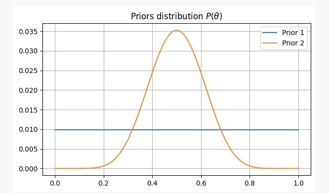
To have different views on this problem, we will solve it under two different prior beliefs:
- You have no prior information about the fairness of the coin, so you assign an equal probability to
p. In this case, we will use what is called a non-informative prior because you haven’t added any information to your beliefs.
For these two scenarios, our prior beliefs will be as follows:
After flipping a coin 10 times, you got heads twice. With this evidence, where are we likely to find our parameter p?
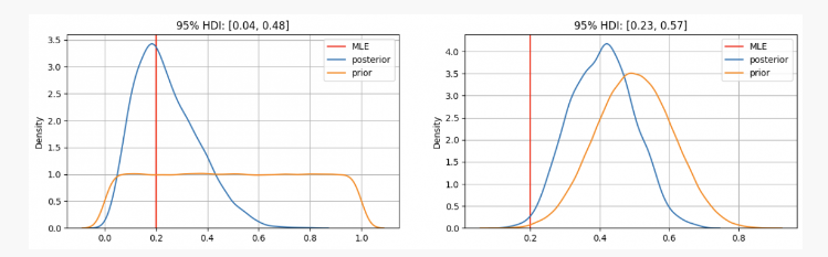
As you can see, in the first case, our prior distribution of parameter p is concentrated at the maximum likelihood estimate (MLE) p=0.2, which is a method similar to that used by the frequency school. The true unknown parameter will be within the 95% confidence interval, between 0.04 and 0.48.
On the other hand, in cases where there is high confidence that parameter p should be between 0.3 and 0.7, we can see that the posterior distribution is around 0.4, much higher than what our MLE gives us. In this case, the true unknown parameter will be within a 95% confidence interval between 0.23 and 0.57.
Therefore, in the first case scenario you would tell your friend with certainty that this coin isn’t fair but in another situation you’d say it’s uncertain whether or not it’s fair.
As you can see even when faced with identical evidence (two heads out of ten tosses), under different prior beliefs results may vary greatly; one advantage of Bayesian statistics over traditional methods lies here: like scientific methodology it allows us to update our beliefs by combining them with new observations and evidence.
END
In today’s article, we saw the origins of Bayesian statistics and its main contributors. Subsequently, there have been many other important contributors to this field of statistics (Jeffreys, Cox, Shannon and so on), reprinted from quantdare.com.