In previous articles, we discussed a common phenomenon in the digital currency market: most digital currencies, especially those that follow the price fluctuations of Bitcoin and Ethereum, often show a trend of rising and falling together. This phenomenon reveals their high correlation with mainstream currencies. However, the degree of correlation between different digital currencies also varies. So how does this difference in correlation affect the market performance of each currency? In this article, we will use the bull market in the second half of 2023 as an example to explore this issue.
The Synchronous Origin of the Digital Currency Market
The digital currency market is known for its volatility and uncertainty. Bitcoin and Ethereum, as the two giants in the market, often play a leading role in price trends. Most small or emerging digital currencies, in order to maintain market competitiveness and trading activity, often keep a certain degree of price synchronization with these mainstream currencies, especially those coins made by project parties. This synchronicity reflects the psychological expectations and trading strategies of market participants, which are important considerations in designing quantitative trading strategies.
Formula and Calculation Method of Correlation
In the field of quantitative trading, the measurement of correlation is achieved through statistical methods. The most commonly used measure is the Pearson correlation coefficient, which measures the degree of linear correlation between two variables. Here are some core concepts and calculation methods:
The range of the Pearson Correlation Coefficient (denoted as r) is from -1 to +1, where +1 indicates a perfect positive correlation, -1 indicates a perfect negative correlation, and 0 indicates no linear relationship. The formula for calculating this coefficient is as follows:
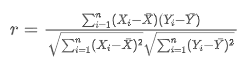
Among them,

and

are the observed values of two random variables,

and

are the average values of these two random variables respectively. Using Python scientific computing related packages, it’s easy to calculate correlation.
Data Collection
This article has collected the 4h K-line data for the entire year of 2023 from Binance, selecting 144 currencies that were listed on January 1st. The specific code to download the data is as follows:
import requests
from datetime import date,datetime
import time
import pandas as pd
import numpy as np
import matplotlib.pyplot as plt

ticker = requests.get('https://fapi.binance.com/fapi/v1/ticker/24hr')
ticker = ticker.json()
sort_symbols = [k['symbol'][:-4] for k insorted(ticker, key=lambda x :-float(x['quoteVolume'])) if k['symbol'][-4:] == 'USDT']

defGetKlines(symbol='BTCUSDT',start='2020-8-10',end='2023-8-10',period='1h',base='fapi',v = 'v1'):
    Klines = []
    start_time = int(time.mktime(datetime.strptime(start, "%Y-%m-%d").timetuple()))*1000 + 8*60*60*1000
    end_time =  min(int(time.mktime(datetime.strptime(end, "%Y-%m-%d").timetuple()))*1000 + 8*60*60*1000,time.time()*1000)
    intervel_map = {'m':60*1000,'h':60*60*1000,'d':24*60*60*1000}
    while start_time < end_time:
        time.sleep(0.5)
        mid_time = start_time+1000*int(period[:-1])*intervel_map[period[-1]]
        url = 'https://'+base+'.binance.com/'+base+'/'+v+'/klines?symbol=%s&interval=%s&startTime=%s&endTime=%s&limit=1000'%(symbol,period,start_time,mid_time)
        res = requests.get(url)
        res_list = res.json()
        iftype(res_list) == listandlen(res_list) > 0:
            start_time = res_list[-1][0]+int(period[:-1])*intervel_map[period[-1]]
            Klines += res_list
        iftype(res_list) == listandlen(res_list) == 0:
            start_time = start_time+1000*int(period[:-1])*intervel_map[period[-1]]
        if mid_time >= end_time:
            break
    df = pd.DataFrame(Klines,columns=['time','open','high','low','close','amount','end_time','volume','count','buy_amount','buy_volume','null']).astype('float')
    df.index = pd.to_datetime(df.time,unit='ms')
    return df

start_date = '2023-01-01'
end_date   = '2023-11-16'
period = '4h'
df_dict = {}

for symbol in sort_symbols:
    print(symbol)
    df_s = GetKlines(symbol=symbol+'USDT',start=start_date,end=end_date,period=period)
    ifnot df_s.empty:
        df_dict[symbol] = df_s

df_close = pd.DataFrame(index=pd.date_range(start=start_date, end=end_date, freq=period),columns=df_dict.keys())
for symbol in symbols:
    df_s = df_dict[symbol]
    df_close[symbol] = df_s.close
df_close = df_close.dropna(how='any',axis=1)
Market Review
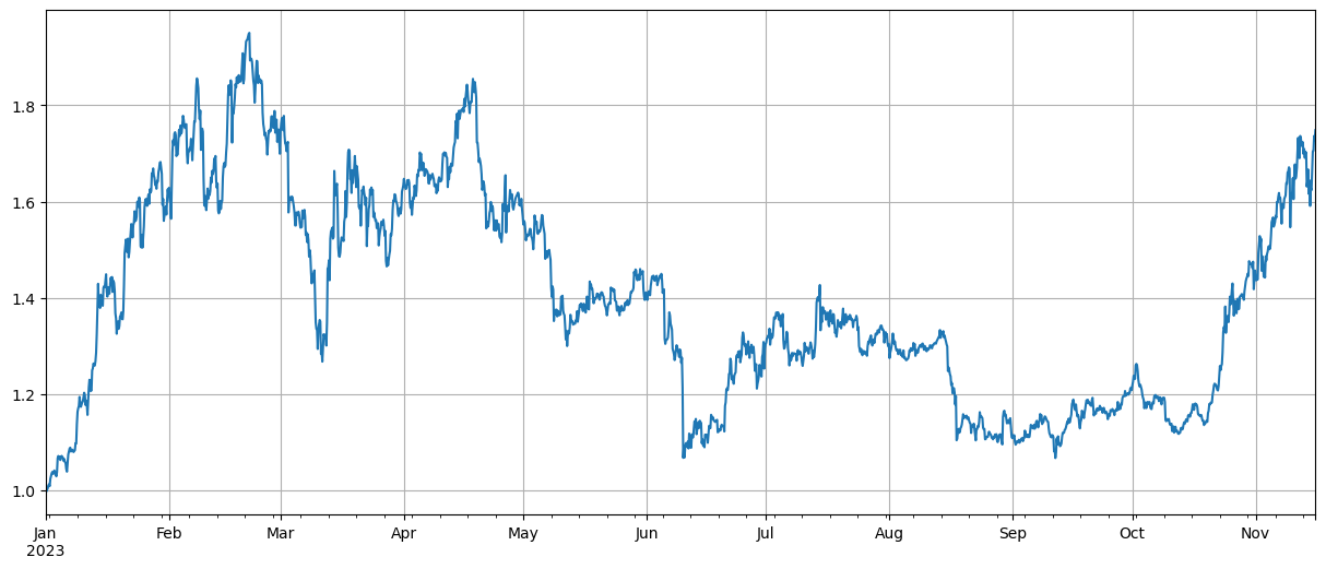
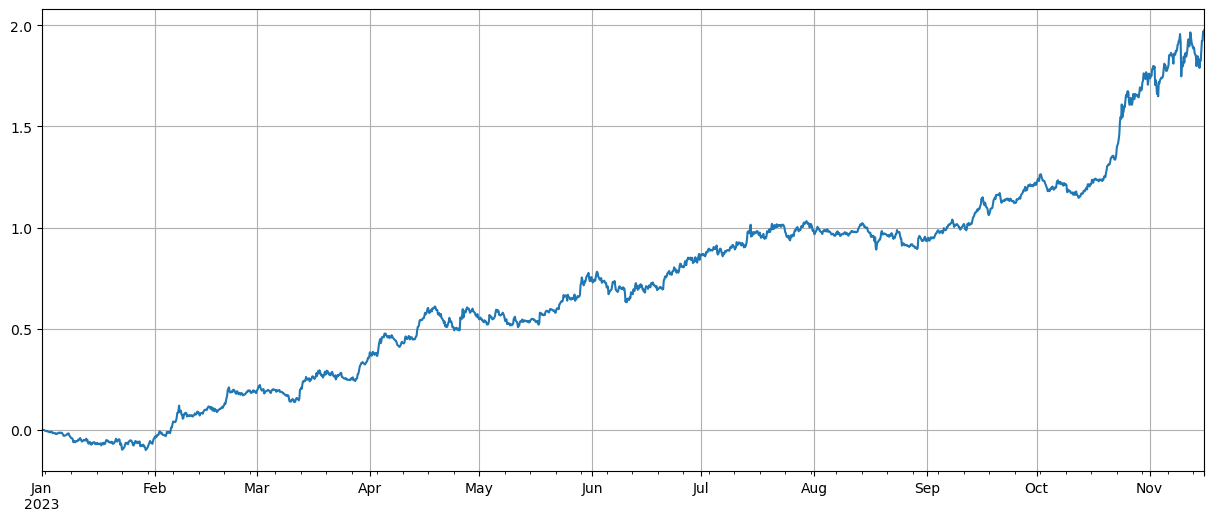
After normalizing the data first, we calculate the index of average price fluctuations. It can be seen that there are two market trends in 2023. One is a significant increase at the beginning of the year, and the other is a major rise starting from October. Currently, it’s basically at a high point in terms of index.
df_norm = df_close/df_close.fillna(method='bfill').iloc[0] #Normalization
total_index = df_norm.mean(axis=1)
total_index.plot(figsize=(15,6),grid=True);
Correlation Analysis
Pandas comes with a built-in correlation calculation. The weakest correlation with BTC price is shown in the following figure. Most currencies have a positive correlation, meaning they follow the price of BTC. However, some currencies have a negative correlation, which is considered an anomaly in digital currency market trends.
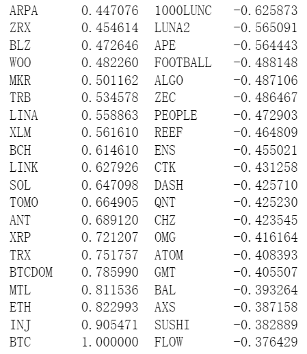
corr_symbols = df_norm.corrwith(df_norm.BTC).sort_values().index
Correlation and Price Increase
Here, the currencies are loosely divided into two groups. The first group consists of 40 currencies most correlated with BTC price, and the second group includes those least related to BTC price. By subtracting the index of the second group from that of the first, it represents going long on the first group while shorting the second one. In this way, we can calculate a relationship between price fluctuations and BTC correlation. Here is how you do it along with results:
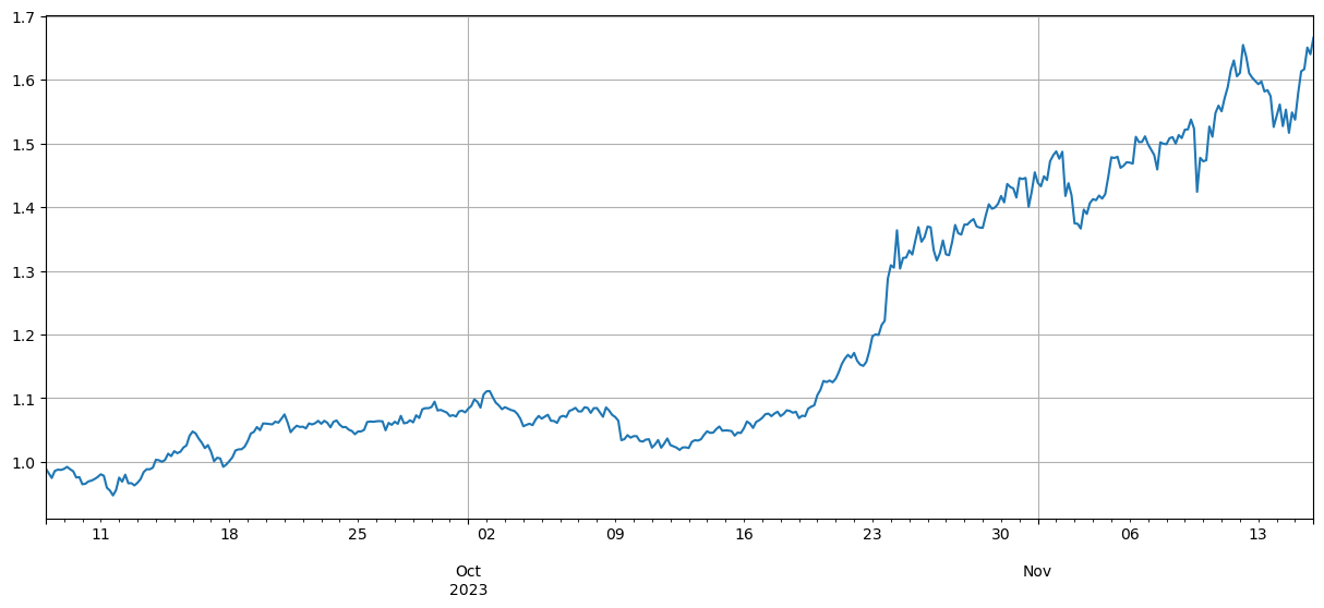
(df_norm[corr_symbols[-40:]].mean(axis=1)-df_norm[corr_symbols[:40]].mean(axis=1)).plot(figsize=(15,6),grid=True);
The results show that the currencies with stronger correlation to BTC price have better increases, and shorting currencies with low correlation also played a good hedging role. The imprecision here is that future data was used when calculating the correlation. Below, we divide the data into two groups: one group calculates the correlation, and another calculates the return after hedging. The result is shown in the following figure, and the conclusion remains unchanged.
Bitcoin and Ethereum as market leaders often have a huge impact on overall market trends. When these cryptocurrencies rise in price, market sentiment usually becomes optimistic and many investors tend to follow this trend. Investors may see this as a signal of an overall market increase and start buying other currencies. Due to collective behavior of market participants, currencies highly correlated with mainstream ones might experience similar price increases. At such times, expectations about price trends can sometimes become self-fulfilling prophecies. On the contrary, currencies negatively correlated with Bitcoin are unique; their fundamentals may be deteriorating or they may no longer be within sight of mainstream investors – there could even exist Bitcoin’s blood-sucking situation where markets abandon them chasing for those able to keep up with rising prices.
corr_symbols = (df_norm.iloc[:1500].corrwith(df_norm.BTC.iloc[:1500])-df_norm.iloc[:1500].corrwith(total_index[:1500])).sort_values().index
Summary
This article discusses the Pearson correlation coefficient, revealing the degree of correlation between different currencies. The article demonstrates how to obtain data to calculate the correlation between currencies and use this data to assess market trends. It reveals that synchronicity in price fluctuations in the digital currency market not only reflects market psychology and strategy, but can also be quantified and predicted through scientific methods. This is particularly important for designing quantitative trading strategies.
There are many areas where the ideas in this article can be expanded, such as calculating rolling correlations, separately calculating correlations during rises and falls, etc., which can yield a lot of useful information.